The effect of integration time on fluctuation measurements:
calibrating an optical trap in the presence of motion blur

Abstract

Dynamical instrument limitations, such as finite detection bandwidth, do not simply add statistical errors to fluctuation measurements, but can create significant systematic biases that affect the measurement of steady-state properties. Such effects must be considered when calibrating ultra-sensitive force probes by analyzing the observed Brownian fluctuations. In this article, we present a novel method for extracting the true spring constant and diffusion coefficient of a harmonically confined Brownian particle that extends the standard equipartition and power spectrum techniques to account for video-image motion blur. These results are confirmed both numerically with a Brownian dynamics simulation, and experimentally with laser optical tweezers.

Published in Optics Express, Vol. 14, Issue 25, pp. 12517–12531 (2006).
©  2006  Optical Society of America

I Introduction

Investigations of micro- to nano-scale phenomena at finite temperature (e.g. single-molecule measurements, microrheology) require a detailed treatment of the Brownian fluctuations that mediate weak interactions and kinetics svoboda1994fam ; mason1995omf ; evans1997dsm ; collin05 . Experimental quantification of such fluctuations are affected by instrument limitations, which can introduce errors in surprising ways. Dynamical limitations, such as finite detection bandwidth, do not simply add statistical errors to fluctuation measurements, but can create significant systematic biases that affect the measurement of steady-state properties such as fluctuation amplitudes and probability densities (e.g. position histograms).

Motion blur, which results from time-averaging a signal over a finite integration time, can create significant problems when imaging fast moving objects. It is particularly relevant when measuring the position fluctuations of a Brownian particle, where even fast detection methods can have long integration times with respect to the relevant time scale, as we will demonstrate in this paper. Instrument bandwidth limitations that arise from motion blur affect a variety of fluctuation-based measurement techniques, including the quantification of forces with magnetic tweezers using lateral fluctuations strick1996ess , and microrheology measurements based on the video-tracking of small particles chen2003rml . The issue of video-image motion blur has recently been addressed in the single-molecule literature yasuda1996dmt and in the field of microrheology, where the static and dynamic errors resulting from video-tracking have been carefully analyzed savin2005sad ; savin2005rfe . However, discussion has been notably absent in the area of ultra-sensitive force-probes, despite the significant effect that it can have on quantitative measurements. This paper focuses on the practical problem of calibration an optical trap by analyzing the confined Brownian motion of a trapped particle ghislain1993sfm ; svoboda1994bao ; gittes1998san ; florin1998pfm ; bergsoerensen2004psa in the presence of video-image motion blur.

In this article, we present a novel method for extracting the true spring constant and diffusion coefficient of a harmonically confined Brownian particle that extends the standard equipartition and power spectrum techniques to account for motion blur. In section (II) we describe how the measured variance of the position of a harmonically trapped Brownian particle depends on the integration time of the detection apparatus, the diffusion coefficient of the bead and the trap stiffness. Next, this theoretical relationship is compared with both simulated data (section (III)) and experimental data using an optical trap (section (IV)). Practical strategies for trap calibration are given in the discussion section (V), where we show that motion blur is not a liability once it is understood, but rather provides valuable information about the dynamics of bead motion. In particular, we show how both the spring constant and the diffusion coefficient can be determined by measuring position fluctuations while varying either the shutter speed of the acquisition system or the confinement strength of the trap.

II Bias in the measured variance of a harmonically trapped Brownian particle

Detection systems, such as video cameras and photodiodes, do not measure the instantaneous position of a particle. Rather, the measured position $X_{m}$ is an average of the true position $X$ taken over a finite time interval, which we call the integration time $W$. In the simplest model,

$$X_{m}(t)=\frac{1}{W}\int_{t-W}^{t}X(t^{\prime})\mathrm{d}{t^{\prime}}\;$$ (1)

where both the measured and true positions of the particle have been expressed as functions of time $t$. More complex situations can be treated by multiplying $X(t^{\prime})$ by an instrument-dependent function within the integral, i.e. by using a non-rectangular integration kernel.

We consider the case of a particle undergoing Brownian motion within a harmonic potential, $U(x)=\frac{1}{2}kx^{2}$. In equilibrium, we expect the probability density of the particle position to be established by the Boltzmann weight $\exp(-U(x)/k_{B}T)$, where $k_{B}$ is the Boltzmann constant and $T$ is the absolute temperature:

$$\rho_{X}(x)=\frac{1}{\sqrt{2\pi k_{B}T/k}}\exp\left(-\frac{kx^{2}}{2k_{B}T}\right)$$ (2)

The variance of the position should then satisfy the equipartition theorem,

$$\text{var}(X)\equiv\left\langle X^{2}\right\rangle-\left\langle X\right\rangle^{2}=\frac{k_{B}T}{k}$$ (3)

However, these equations do not hold for the measured position $X_{m}$. In particular, motion blur introduces a systematic bias in the measured variance,

$$\text{var}(X_{m})\leq\text{var}(X)$$ (4)

Following standard techniques (e.g. oppenheim1996ss ), the necessary correction can be calculated precisely as a function of the spring constant $k$, the friction factor of the particle $\gamma$, and the integration time of the imaging device $W$ yasuda1996dmt ; savin2005sad ; savin2005rfe . First, we define the dimensionless parameter $\alpha$ by expressing the exposure time $W$ in units of the trap relaxation time $\tau=\gamma/k$, i.e.

$$\alpha\equiv\frac{W}{\tau}$$ (5)

Note that $\alpha$ can also be expressed in terms of the diffusion coefficient $D$ by using the Einstein relation $\gamma=k_{B}T/D$, i.e. $\alpha=WDk/(k_{B}T)$. Then as presented in appendix (A), the measured variance is given by:

$$\text{var}(X_{m})=\text{var}(X)S(\alpha)$$ (6)

where $S(\alpha)$ is the motion blur correction function

$$S(\alpha)=\frac{2}{\alpha}-\frac{2}{\alpha^{2}}\left(1-\exp(-\alpha)\right)$$ (7)

III Numerical studies

To verify Eq. (6) numerically, we use a simple Brownian dynamics ermak1978bdh simulation of a bead fluctuating in a harmonic potential. For each time step $\Delta t$, the change in the bead position $\Delta x$ is given by a discretization of the overdamped Langevin equation:

$$\Delta x=\frac{D}{k_{B}T}f_{\text{det}}+\delta x(\Delta t)$$ (8)

where $\delta x(\Delta t)$ is a Gaussian random variable with $\left\langle\delta x\right\rangle=0$ and $\bigl{\langle}\left(\delta x\right)^{2}\bigr{\rangle}=2D\Delta t$, and the deterministic force $f_{\text{det}}=-kx$ corresponds to a harmonic potential as in our calculation. Motion blur is simulated by time-averaging the simulated bead positions over a finite integration time $W$. To minimize errors due to discretization, the simulation sampling time is much smaller than both $W$ and $\Gamma/m$.

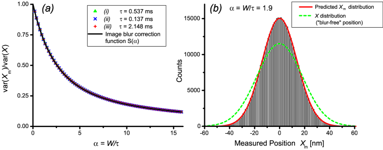
Figure 1: (a) Brownian dynamics simulation results for measured variance as a function of exposure time. Data has been rescaled and plotted alongside $S(\alpha)$, the motion blur correction function of Eq. (7), showing excellent agreement within the expected error. The step size of the simulation is by $1\mu\text{s}$, which is less than $0.01\tau$ for all three simulations. The different simulation settings are: (i) $1.6\>\mu\text{m}$ bead radius, $k=0.05$ pN/nm, $\tau=0.537\>\text{ms}$, (ii) $0.4\>\mu\text{m}$ bead radius, $k=0.05$ pN/nm, $\tau=0.134\>\text{ms}$, (iii) ($1.6\>\mu\text{m}$ bead radius, $k=0.0125$ pN/nm, $\tau=2.148\>\text{ms}$) (b) Histogram of measured positions for simulation run (c) for an exposure time of 4 ms. It is a Gaussian distribution as expected wang1945tbm . The normal curve with the predicted variance is superimposed showing excellent agreement. The expected distribution for an ideal “blur-free” measurement system is superimposed as a dotted line.

Fig. 1(a) shows the simulation results for 3 different bead and spring constant settings as described in the caption. Agreement with the motion blur correction function $S(\alpha)$ of Eq. (7) is within the fractional standard error of the variance, $\sim\sqrt{2/N}$ kenney1951msp . We observe in Fig. 1(b) that the distribution of measured positions is a Gaussian random variable with variance $\text{var}(X_{m})<k_{B}T/k$, and is therefore fully characterized by the mean (trap center) and the measured variance calculated in Eq. (6).

IV Experimental verification

IV.1 Instrument description

The optical trap is formed by focusing 1064 nm near-IR laser light (Coherent Compass 1064-4000M Nd:YVO₄ laser) through a high numerical aperture oil immersion objective (Zeiss Plan Neofluar 100x/1.3) into a closed, water filled chamber. Laser power is varied with a liquid-crystal power controller (Brockton Electro-Optics). This optical tweezers system is integrated into an inverted light microscope (Zeiss Axiovert S100).

The trapped bead is imaged with transmitted bright field illumination provided by a 100 W halogen lamp (Zeiss HAL 100). The image is observed with a high-speed cooled CCD camera with adjustable exposure time (Cooke high performance SensiCam) connected to a computer running custom data acquisition software heinrich_software1 . Each video frame is processed in real-time to determine the position of the trapped bead. Fast one-dimensional position detection is accomplished by analyzing the intensity profile of a single line passing through the bead center. To increase the signal to noise ratio and the frame rate, the camera bins (i.e. spatially integrates) several lines about the bead center (32 in this experiment) to form the single line used in analysis. A third order polynomial is fit to the two minima corresponding to the one-dimensional “edges” of the bead, giving sub-pixel position detection with a measured accuracy of about 2 nm.

Tracking errors can be included in the measured variance by adding the parameter $\varepsilon^{2}$ to Eq. (6), i.e.

$$\text{var}(X_{m})=\frac{2k_{B}T}{k}\left(\frac{\tau}{W}-\frac{\tau^{2}}{W^{2}}(1-\exp(-W/\tau))\right)+\varepsilon^{2}$$ (9)

$\varepsilon^{2}$ can be interpreted as the measured variance of a stationary particle, provided there are no correlations between the tracking error and the measured positions. A detailed treatment of such particle tracking errors is provided in reference savin2005sad , where the authors also stress the importance of using identical conditions of noise and signal quality when comparing the $\varepsilon^{2}$ parameter between different experimental runs. Care was taken to achieve these conditions as is described below.

IV.2 Experimental conditions

The sample chamber was prepared with pure water and polystyrene beads (Duke Scientific certified size standards 4203A, 3.063 $\mu$m $\pm$ 0.027 $\mu$m). Experiments were performed by holding a bead in the optical trap and varying the power and the exposure time. The bead was held 30 $\mu$m from the closest surface, and the lamp intensity was varied with exposure time to ensure a similar intensity profile for each test. This ensured that the noise and signal quality between experimental runs was very similar, as validated by the results. For each test, both edges of the bead in one dimension were recorded and averaged to estimate the center position.

IV.3 Experimental Results

The one-dimensional variance of a single bead in an optical trap was measured at various laser powers and exposure times. Low frequency instrument drift was filtered out as described in Appendix B. For each power, measured variance vs. exposure time data was fit with Eq. (9) to yield values for the spring constant $k$, friction factor $\gamma$, and tracking error $\varepsilon^{2}$. Error estimates in the variance were calculated from the standard error due to the finite sample size, and variations due to vertical drift.

Error in the fitting parameters indicate that the best estimates for $\gamma$ and $\varepsilon^{2}$ occur at the lowest and highest powers, respectively. These estimates both agree within 2% of the error weighted average for all powers. For the nominal bead size, $\gamma$ agrees with the Stokes’ formula calculation to within 11%, indicating a slightly smaller bead or lower water viscosity than expected. Additionally, the estimate of tracking error $\varepsilon$ determined from the fit compares favorably with the standard deviation in position of a stuck bead, differing by about half a nanometer.

For a single bead observed under identical measurement conditions, $\gamma$ and $\varepsilon^{2}$ are expected to remain essentially constant as the laser power is varied. Good consistency was found between the determined values of $\varepsilon^{2}$ from different experimental runs, due to the protocol of matching the signal strength between tests. While laser heating could cause $\gamma$ to decrease with increasing power, this effect should be small for the $<$ 500 mW powers used here peterman2003lih ; celliers2000mlh , so this effect was neglected.

Holding $\gamma$ and $\varepsilon^{2}$ constant for all powers, the raw data was re-fit with Eq. (9) to yield $k$. The data for all 4 powers was error-corrected by subtracting $\varepsilon^{2}$ and was rescaled according to Eq. (6) and Eq. (7). This non-dimensionalized data is plotted alongside the motion blur correction function in Fig. 2, showing near-perfect quantitative agreement. This exceptional agreement further validates our treatment of $\gamma$ and $\varepsilon^{2}$. A plot of spring constant vs. dimensionless power is shown in Fig. 3, demonstrating the discrepancy between the blur-corrected spring constant and naïve spring constant for different integration times. Even for a modest spring constant of 0.03 pN/nm and a reasonably fast exposure time of 1 ms, the expected error is roughly 50%. We also note that the blur-corrected spring constant increases linearly with laser power as expected from optical-trapping theory. Once confirmed for a given system, this linearity can be exploited to determine not only the spring constant as a function of power but also the diffusion coefficient of the bead. This is discussed in subsection (V.3), and presented in Fig. 3.

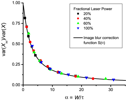
Figure 2: Fractional variance $(\text{var}(X_{m})/\text{var}(X))$ vs. dimensionless exposure time $\alpha=W/\tau$ for experimental optical trap data at 4 different powers. Overlaid on the data is the motion blur correction function $S(\alpha)$ given by Eq. (7).

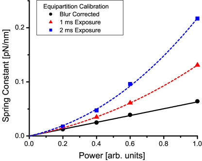
Figure 3: Spring constant vs. power for a single bead in the optical trap. The naïve equipartition measured spring constant with 1 ms and 2 ms exposure times (red triangles and blue squares, respectively) is compared with the blur corrected spring constant (black circles). The dashed blue and red lines going through the uncorrected data represent non-linear fits to the blur model assuming a linear relationship between $k$ and laser power, i.e. $k=cP$, as discussed in subsection (V.3). The values obtained from these fits for $c$ and $\gamma$ agree within error with the “black circle” values obtained by varying the exposure time.

When the data acquisition rate is sufficiently high relative to $1/\tau=k/\gamma$, it is feasible to calibrate the trap using the bead position power spectrum, allowing comparisons to the previous results at low laser power. Power spectrum fitting with the blur-corrected and aliased expression (Eq. (23)) at the lowest power yielded both a spring constant and friction factor that agree with the blur-corrected equipartition values to within 1%. Fits of the same data using the naïve expression (Eq. (13), not corrected for exposure time or aliasing) provided slightly worse results, overestimating the spring constant by 3% and the friction factor by 7%. (See Appendix C for procedural details.)

For an additional check that does not rely on fluctuations, a purely mechanical test was performed and compared with the corrected power spectrum fit. This test consisted of a bead drop experiment to determine the bead radius and friction factor, and a trap recoil experiment to determine the spring constant. The bead drop was performed by releasing a bead and recording its average velocity over a known distance. The trap recoil experiment was performed by measuring the exponential decay of the same bead as it returned to the trap center after deviation in one dimension. This mechanical test agrees with the corrected power spectrum fit to within 5% for the determination of both the spring constant and the friction factor.

V Discussion: Practical suggestions for calibrating an optical trap

In this section, we present some practical techniques for measuring the spring constant $k$ and diffusion coefficient $D$ of a harmonically confined Brownian particle. We will assume that the temperature $T$ is known. The approaches here are generic, and can be used even if the confining potential is not an optical trap (e.g. beads embedded in a gel, etc.) We will continue to treat the measured position as an unweighted time average of the true position over the integration time $W$ (Eq. (1)), which is consistent with the experimental results for our detection system. In other situations, e.g. if the rise and fall time are not negligible relative to the exposure time, these equations and ideas can be readily generalized as noted in section (II).

V.1 Determining $k$ from $D$ and $W$.

If the diffusion coefficient $D$ of the confined particle and the integration time $W$ of the instrument is known, the correct spring constant $k$ can be directly obtained from the measured variance $\text{var}(X_{m})$ by using equation 6. If the tracking error $\varepsilon$ is significant, $\varepsilon^{2}$ should first be subtracted from the measured variance as in equation 9. While we cannot in general isolate $k$ in this transcendental equation, it can easily be found numerically by utilizing a standard root-finding method. Alternatively, an approximate closed form solution for $k$ is derived in Appendix D.

V.2 Determining $k$ and $D$ by varying $W$

Even if the data acquisition rate of the system is not fast enough to permit a blur-corrected power spectrum fit (as described in Appendix C), $k$ and $D$ can still be determined by measuring the variance at different shutter speeds and fitting to the blur-corrected variance function. This technique is demonstrated in the experimental results section, and yields accurate measurements provided the integration time is not too much larger than the trap relaxation time ($\alpha$ is not much larger than 1). Practically speaking, this is a useful technique, as the maximum shutter speed of a camera is often much faster than the maximum data acquisition speed (e.g. it is much easier to obtain a video camera with a 0.1 ms shutter speed than a camera with a frame rate of 10 kHz). Furthermore, this approach for quantifying the power spectrum from the blur is quite general, and could be used in other systems. As long as the form of the power spectrum is known, the model parameters could be determined by measuring the total variance over a suitable spectrum of shutter speeds.

V.3 Determining $k$ and $D$ by varying $k$

Other approaches are possible if the confinement of the particles can be varied in a controlled way, i.e. by varying the laser power of the optical trap. If the spring constant varies linearly with laser power, (which is typically true and was confirmed for our system in subsection (IV.3)), the first observation is that the spring constant only needs to be measured at a single laser power, as it can be extrapolated to other laser powers. Typically calibration should be done at a low power, as this usually increases the accuracy of both the power spectrum fit and the blur correction technique.

Linearity between the spring constant and laser power can be further exploited to determine both $k$ and $D$ by measuring the variance of a trapped bead at different laser powers but with the same shutter speed. Such data can be fit to the blur model (equation 6, recalling that $\alpha=WDk/(k_{B}T)$) by introducing an additional fitting parameter $c$ that relates the laser power $P$ to the spring constant, i.e. we make the substitution $k=cP$, and perform a non-linear fit to $\text{var}(X_{m})$ vs. power data in order to determine $c$ and $D$. Equivalently, we can express the naïve spring constant $k_{m}=k_{B}T/\text{var}(X_{m})$ as a function of $c$ and $P$, and perform a fit to $k_{m}$ vs. $P$ data as shown in Fig. 3 of the experimental results subsection (IV.3), where the viability of this method is demonstrated.

V.4 Design strategies for using the blur technique

When using these motion blur techniques to characterize the dynamics of confined particles, we reiterate that it is the shutter speed and not the data acquisition speed that limits the dynamic range of a measurement. Thus, even inexpensive cameras with fast shutter speeds can make dynamical measurements without requiring the investment of a fast video camera. Alternative methods for controlling the exposure time are the use of optical shutters or strobe lights.

VI Conclusions

We have experimentally verified a relationship between the measured variance of a harmonically confined particle and the integration time of the detection device. This yields a practical prescription for calibrating an optical trap that corrects and extends both the standard equipartition and power spectrum methods. By measuring the variance at different shutter speeds or different laser powers, the true spring constant can be determined by application of the motion blur correction function of Eq. (7). Additionally, this provides a new technique for determining the diffusion coefficient of a confined particle from time-averaged fluctuations.

The dramatic results from our experiment indicate that integration time of the detection device cannot be overlooked, especially with video detection. Furthermore, we have shown that motion blur need not be a detriment if it is well understood, as it provides useful information about the dynamics of the system being studied.

Appendix A Calculation of the measured variance of a harmonically trapped Brownian particle

In this appendix, a derivation of the motion blur correction function Eq. (7) is presented. This quantifies how the measured variance depends upon the spring constant $k$, the diffusion coefficient of the particle $D$, and the integration time of the imaging device $W$ (notation is as introduced in section (II)). The derivation follows standard techniques (e.g. oppenheim1996ss ) and is similar to calculations presented in references yasuda1996dmt ; savin2005sad ; savin2005rfe ; wang1945tbm . For completeness, we present the calculation in two different ways: (A.1) a frequency-space calculation that convolves the true particle trajectory with the appropriate moving-average filter, and (A.3) a real-space calculation using Green’s functions. An expression for the modified power spectrum of the harmonically confined bead that accounts for the effects of filtering and aliasing is included in the frequency-space calculation (see subsection (A.2))

A.1 Frequency-space calculation

The measured trajectory of a particle in the presence of motion blur $X_{m}(t)$ can be calculated by convolving the true trajectory $X(t)$ with a rectangular function,

$$X_{m}(t)=X(t)\ast H(t)\equiv\int X(t^{\prime})H(t-t^{\prime})\mathrm{d}{t^{\prime}}\;$$ (10)

where $H(t)$ is defined by:

$$H(t)=\left\{\begin{array}[]{cl}\frac{1}{W}&0<t\leq W\\ 0&\text{elsewhere}\end{array}\right.$$ (11)

The integral is taken over the full range of values (i.e. $t^{\prime}$ is integrated from $-\infty$ to $+\infty$), which is our convention whenever limits are not explicitly written. The width of the rectangle $W$ is simply the integration time as previously defined. This convolution acts as an ideal moving average filter in time, and is consistent with the integral expression for $X_{m}(t)$ given in Eq. (1).

Taking the power spectrum of Eq. (10) yields:

$$P_{m}(\omega)\equiv\left|\tilde{X}_{m}(\omega)\right|^{2}=\left|\tilde{X}(\omega)\right|^{2}\left|\tilde{H}(\omega)\right|^{2}$$ (12)

Where the Fourier transform is denoted by a tilde, e.g. $\tilde{X}(\omega)=\int X(t)\exp(i\omega t)\mathrm{d}{t}\;$, and $\omega$ is the frequency in radians/second. The theoretical power spectrum $P(\omega)$ is given by:

$$P(\omega)\equiv\left|\tilde{X}(\omega)\right|^{2}=\frac{2\gamma k_{B}T}{\gamma^{2}\omega^{2}+k^{2}}$$ (13)

where $\gamma$ is the friction factor of the particle, and is related to the diffusion coefficient by the Einstein relation $\gamma=k_{B}T/D$. This power spectrum has been well-described previously svoboda1994bao ; wang1945tbm ; gittes1998san , and is derived in section (A.3).

The power spectrum of the moving average filter can be expressed as a squared sinc function:

$$\left|\tilde{H}(\omega)\right|^{2}=\left({\frac{\sin(\omega W/2)}{\omega W/2}}\right)^{2}$$ (14)

Using Parseval’s Theorem and integrating the power spectrum $P(\omega)$ yields the true variance of $X(t)$,

$$\text{var}(X)=\frac{1}{2\pi}\int P(\omega)\mathrm{d}{\omega}\;=\frac{k_{B}T}{k}$$ (15)

which is in agreement with the equipartition theorem. Similarly, we calculate the measured variance $\text{var}(X_{m})$ as a function of the exposure time $W$ and the friction factor $\gamma$ by integrating the power spectrum of the measured position (Eq. (12)):

$$\text{var}(X_{m}) = \frac{1}{2\pi}\int P_{m}(\omega)\mathrm{d}{\omega}\;$$ (16)

$$= \frac{2k_{B}T}{k}\left(\frac{\tau}{W}-\frac{\tau^{2}}{W^{2}}(1-\exp(-W/\tau))\right)$$ (17)

where $\tau=\gamma/k$, the trap relaxation time. Writing this formula in terms of the dimensionless exposure time,

$$\alpha\equiv\frac{W}{\tau}$$ (18)

and the variance of the true bead position $\text{var}(X)=k_{B}T/k$ yields:

$$\text{var}(X_{m})=\text{var}(X)S(\alpha)$$ (19)

where $S(\alpha)$ is the motion blur correction function:

$$S(\alpha)=\frac{2}{\alpha}-\frac{2}{\alpha^{2}}\left(1-\exp(-\alpha)\right)$$ (20)

A.2 Blur-corrected filtered power spectrum

Often, trap calibration is performed by fitting the power spectrum of a confined particle. Here we provide a modification to the standard functional form $P(\omega)$ that accounts for both exposure time effects and aliasing. Combining expressions 12, 13 and 14, we can see the effect of exposure time on the measured power spectrum:

$$P_{m}(\omega)=\frac{2\gamma k_{B}T}{\gamma^{2}\omega^{2}+k^{2}}\left({\frac{\sin(\omega W/2)}{\omega W/2}}\right)^{2}$$ (21)

Additionally, the effect of aliasing can be accounted for:

$$P_{\text{aliased}} = \sum_{n=-\infty}^{+\infty}{P_{m}(\omega+n\omega_{s})}$$ (22)

$$= \sum_{n=-\infty}^{+\infty}\frac{2\gamma k_{B}T}{\gamma^{2}(\omega+n\omega_{s})^{2}+k^{2}}\left(\frac{\sin((\omega+n\omega_{s})W/2)}{(\omega+n\omega_{s})W/2}\right)^{2}$$ (23)

where $\omega_{s}$ is the angular sampling frequency (i.e. the data acquisition rate times $2\pi$). Aliasing changes the shape of the power spectrum, so neglecting it when fitting can cause errors. The sum in Eq. (23) can be calculated numerically and fit to experimental data. It is typically sufficient to calculate only the first few terms.

It is important to note that aliasing does not affect our result for the measured variance, Eq. (17). Aliasing shifts power into the wrong frequencies, but does not change the integral of the power. Hence, $\text{var}(X_{m})$ is unchanged. A detailed discussion of power spectrum calibration with an emphasis on photodiode detection systems is given in reference bergsoerensen2004psa .

A.3 Real-space calculation

Since a Brownian particle follows a random trajectory $X(t)$, the measured position $X_{m}$ is a random function of the true position of the particle at the start of the integration time, i.e.

$$X_{m}(x_{0})=\frac{1}{W}\int_{0}^{W}X(t\mid x_{0})\mathrm{d}{t}\;$$ (24)

where $X(t\mid x_{0})$ is the actual position of the bead at time $t$ given that it is at position $x_{0}$ at time zero, and $W$ is the integration time as defined previously. In other words, even with knowledge of the initial particle position, it is not possible to predict what the measured position will be. However, the distribution of $X_{m}$ is well-defined, and one can determine its moments.

The variance of the measured position is given by

$$\text{var}(X_{m})\equiv\left\langle X_{m}(X)^{2}\right\rangle-\left\langle X_{m}(X)\right\rangle^{2}$$ (25)

Notice that to calculate the ensemble average $\left\langle\dots\right\rangle$, we must average over both the random initial position $X$, and the measured position for a given initial position $X_{m}(x)$. For the harmonic potential $U(x)=\frac{1}{2}kx^{2}$, $\left\langle X_{m}(X)\right\rangle=0$ by symmetry, so the variance reduces to

$$\text{var}(X_{m})=\int\rho_{X}(x_{0})\ \left\langle X_{m}(x_{0})^{2}\right\rangle\ \mathrm{d}{x_{0}}\;$$ (26)

where $\rho_{X}(x_{0})$ is the probability density of the initial position, and the integral is taken over all space (consistent with our previously stated convention). In equilibrium, $\rho_{X}(x_{0})$ is simply the Boltzmann distribution given in Eq. (2).

Using Eq. (24), we express $\left\langle X_{m}(x_{0})^{2}\right\rangle$ as the double integral

$$\left\langle X_{m}(x_{0})^{2}\right\rangle =\left\langle\frac{1}{W^{2}}\int_{0}^{W}\!\!\!\int_{0}^{W}X(t_{1}\mid x_{0})X(t_{2}\mid x_{0})\ \mathrm{d}{t_{1}}\;\mathrm{d}{t_{2}}\;\right\rangle$$ (27)

$$=\frac{2}{W^{2}}\int_{0}^{W}\!\!\!\int_{0}^{t_{2}}\left\langle X(t_{1}\mid x_{0})X(t_{2}\mid x_{0})\right\rangle_{t_{2}>t_{1}}\ \mathrm{d}{t_{1}}\;\mathrm{d}{t_{2}}\;$$ (28)

In the second step, the ensemble average is brought into the integral, and the averaging condition $t_{2}>t_{1}$ is added, which changes the limits of integration.

The time-ordered auto-correlation function $\left\langle X(t_{1})X(t_{2})\right\rangle_{t_{2}>t_{1}}$ can be calculated using the Green’s function of the diffusion equation for a harmonic potential, $\rho\left(x,t\mid x_{0},t_{0}\right)$. The Green’s function represents the probability density for finding the particle at position $x$ at time $t$ given that it is at $x_{0}$ at time $t_{0}$. It can be found by solving the diffusion equation

$$\frac{\partial{\rho}}{\partial{t}}=D\frac{\partial^{2}{\rho}}{\partial{x}^{2}}+\frac{D}{k_{B}T}\frac{\partial{\rho}}{\partial{x}}kx+\frac{D}{k_{B}T}\rho k$$ (29)

with the initial conditions $\rho(x,t_{0})=\delta(x-x_{0})$. The solution to this problem is well-known doi1986tpd ; wang1945tbm and is given by:

$$\rho\left(x,t\mid x_{0},t_{0}\right)=\frac{1}{\sqrt{2\pi k_{B}TV(t-t_{0})/k}}\exp\left(-\frac{k\left(x-x_{0}\exp(-(t-t_{0})/\tau)\right)^{2}}{2k_{B}TV(t-t_{0})}\right)$$ (30)

where we have defined the dimensionless function:

$$V(t)=1-\exp(-2t/\tau)$$ (31)

As before $\tau=\ k_{B}T/(kD)=\gamma/k$. Notice that this is simply a spreading Gaussian distribution with the mean given by the deterministic (non-Brownian) position of a particle connected to a spring in an overdamped environment, and with a variance that looks like free diffusion at short time scales (i.e. initially increasing as $2D(t-t_{0})$), but exponentially approaching the equilibrium value of $k_{B}T/k$ on longer time scales.

The time-ordered auto-correlation function can be written as follows:

$$\left\langle X(t_{1})X(t_{2})\right\rangle_{t_{2}>t_{1}}=\int\!\!\!\int x_{1}x_{2}\rho(x_{1},t_{1}\mid x_{0},0)\rho(x_{2},t_{2}\mid x_{1},t_{1})\mathrm{d}{x_{1}}\;\mathrm{d}{x_{2}}\;$$ (32)

Putting in the Green’s function of Eq. (30) and evaluating the integrals gives the result:

$$\left\langle X(t_{1})X(t_{2})\right\rangle_{t_{2}>t_{1}}=x_{0}^{2}\exp(-(t_{2}+t_{1})/\tau)+\frac{k_{B}T\ V(t_{1})}{k}\exp(-(t_{2}-t_{1})/\tau)$$ (33)

where $V(t)$ and $\tau$ are as defined above.

Carrying out the double time integral in Eq. (27), followed by the integral over the initial position $x_{0}$ of Eq. (26) we obtain the final result for the measured variance:

$$\text{var}(X_{m})=\frac{2k_{B}T}{k}\left(\frac{\tau}{W}-\frac{\tau^{2}}{W^{2}}(1-\exp(-W/\tau))\right)$$ (34)

This reproduces the result of the frequency-space calculation presented in Eq. (17). The ideal power spectrum can be obtained from the position auto-correlation function of Eq. (33). We determine the long-time limit of the auto-correlation function by letting $t_{1}\gg\tau$, which yields the simplified equation:

$$\left\langle X(t_{1})X(t_{2})\right\rangle=\frac{k_{B}T}{k}\exp(-\left|t_{2}-t_{1}\right|/\tau)$$ (35)

Next, by taking the Fourier transform of this equation with respect to $(t_{2}-t_{1})$ we obtain the standard result of Eq. (13).

Appendix B High-pass filtering in variance measurements

Calculation of the variance requires special attention, since low frequency noise or drift can inflate the variance dramatically, causing an underestimation of the spring constant. A high pass filter can be used to remove low frequency noise, but the use of any ideal filter lowers the variance by neglecting the contribution from the removed frequencies (note Eq. (15)).

To reliably estimate the variance while accounting for low frequency drift, we first progressively high-pass filter the data over a range of increasing cut-off frequencies. A plot of measured variance vs. cutoff frequency (Fig. 4) clearly shows a linear trend at frequencies below the corner frequency (f_c=k/2$\pi\gamma)$. However, as the filtering frequencies approach zero, drift causes the measured variance to increase beyond its expected value. By applying a linear fit and extrapolating to the 0 Hz cutoff, we can reliably estimate the “drift-free” variance of bead position.

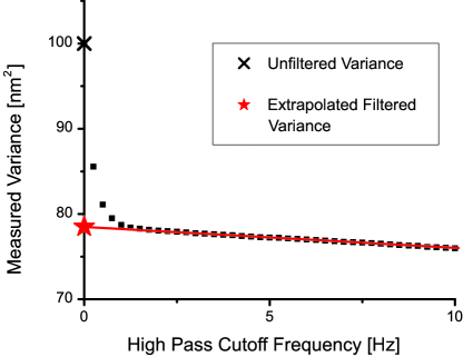
Figure 4: Experimentally measured variance as a function of the high pass filter cutoff frequency shows a linear relation (line), which can be extrapolated to 0 Hz to reliably estimate the drift-free variance. The variance without filtering (cross) is $100\>\text{nm}^{2}$, while the extrapolated variance (star) is $78.5\>\text{nm}^{2}$

Appendix C Experimental power spectrum calibration

Power spectrum calibrations were performed by fitting the one-sided power spectrum with Eq. (23). The original 65536 data points taken at $\sim$1500 samples per second were blocked into 128 non-overlapping segments. The power spectrum of the blocks were calculated separately and averaged to produce the data in Fig. 5. This procedure is well described in the literature gittes1998san ; bergsoerensen2004psa . This data was fit with the blur-corrected and aliased model of Eq. (23) and compared with the commonly used non-corrected power spectrum of Eq. (13), both with and without aliasing. The quality of the fit to Eq. (23) was further investigated by examining the fractional deviation in the power (the measured data divided by the model fit) as in reference bergsoerensen2004psa . A scatter plot and histogram of the fractional deviation is presented in Fig. 6. The histogram agrees well with a Gaussian distribution with a standard deviation of $1/\sqrt{128}$ (see reference bergsoerensen2004psa for a thorough discussion of power-spectrum fitting, including the expected scatter from unity).

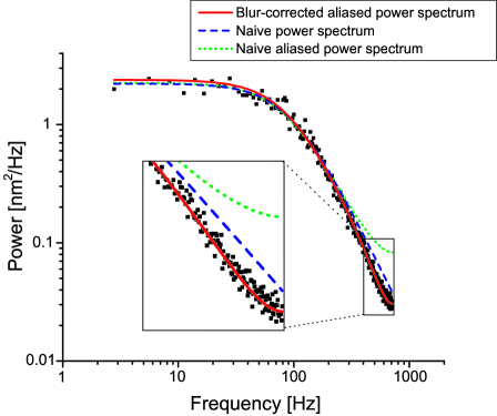
Figure 5: A log-log plot of the one-sided power spectrum (dots) for a trapped bead, with theoretical models produced from a least squares fit to the data (blur-corrected and aliased, Eq. (23) solid line; naïve, Eq. (13) blue dashed line; naïve aliased, green dotted line). The effect of the motion blur correction function $S(\alpha)$ is readily apparent from the clear discrepancy between the solid red and dotted green lines.

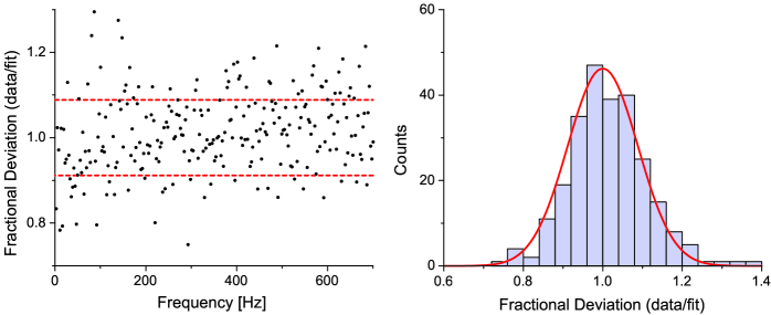
Figure 6: Fractional deviation of the power spectrum data obtained by dividing the experimentally measured values (dots in Fig. 5) by the fit obtained with the blur-corrected and aliased model (solid red line in Fig. 5). Left: Scatter plot demonstrating the quality of the fit; the two dashed red lines indicate the estimated standard deviation from unity of $1/\sqrt{128}$ bergsoerensen2004psa . Right: Histogram of the fractional deviation data overlaid with a Gaussian distribution with a standard deviation of $1/\sqrt{128}$ (solid red line).

Accounting for tracking error in the power spectrum fit is more difficult than in the equipartition case, requiring knowledge of the frequency dependence of the error. To investigate this in the current study, the power spectrum of a stationary bead was subtracted from the calibration power spectrum. We found that the fit parameters remained practically unchanged (within 2%), allowing us to neglect tracking error in our power spectrum fits at low power. It should be noted that in other situations (e.g. different bead size or power), modifications to the power spectrum due to tracking error could be significant.

Appendix D Approximate analytical expression for $k$

When $W$ is not significantly larger than the trap relaxation time, i.e. $\alpha=W/\tau=Wk/\gamma$ is not much larger than 1, an approximate version of equation 6 can be inverted to give a closed form solution for $k$. First, we use a Padé approximation to express the motion blur correction function as:

$$S(\alpha)\approx\frac{1-2\alpha/15+\alpha^{2}/60}{1+\alpha/5}$$ (36)

Substituting this expression into equation 6 yields a quadratic equation that is easily solved for $k$. This results in the following approximation for the true spring constant:

$$k\approx\frac{30\,k_{B}T}{2DW+15\,\text{var}(X_{m})+\left[225\,\text{var}(X_{m})^{2}+240DW\text{var}(X_{m})-11D^{2}W^{2}\right]^{1/2}}$$ (37)

The Padé approximation is good to within 3% for $\alpha<3$, which corresponds to a blur correction factor of $S(3)\doteq 0.46$. In other words, if the uncorrected equipartition method gives a spring constant which is within a factor of 2 of the true value, this approximation formula should be accurate to within 3%, as we have tested numerically.

References

- (1) K. Svoboda, P.P. Mitra, and S.M. Block, “Fluctuation analysis of Motor Protein Movement and Single Enzyme Kinetics,” Proc. Natl. Acad. Sci. USA 91, 11782–11786 (1994).
- (2) T.G. Mason and D.A. Weitz, “Optical Measurements of Frequency-Dependent Linear Viscoelastic Moduli of Complex Fluids,” Phys. Rev. Lett. 74, 1250–1253 (1995).
- (3) E. Evans and K. Ritchie, “Dynamic strength of molecular adhesion bonds,” Biophys. J. 72, 1541–1555 (1997).
- (4) D. Collin, F. Ritort, C. Jarzynski, S.B. Smith, I. Tinoco, Jr., and C. Bustamante, “Verification of the Crooks fluctuation theorem and recovery of RNA folding free energies,” Nature (London)437, 231–234 (2005).
- (5) T.R. Strick, J.F. Allemand, D. Bensimon, A. Bensimon, and V. Croquette, “The elasticity of a single supercoiled DNA molecule.” Science 271, 1835–1837 (1996).
- (6) D.T. Chen, E.R. Weeks, J.C. Crocker, M.F. Islam, R. Verma, J. Gruber, A.J. Levine, T.C. Lubensky, and A.G. Yodh, “Rheological Microscopy: Local Mechanical Properties from Microrheology,” Phys. Rev. Lett. 90, 108301 (2003).
- (7) R. Yasuda, H. Miyata, and K. Kinosita, Jr., “Direct measurement of the torsional rigidity of single actin filaments,” J. Mol. Biol. 263, 227–236 (1996).
- (8) T. Savin and P.S. Doyle, “Static and Dynamic Errors in Particle Tracking Microrheology,” Biophys. J. 88, 623–638 (2005).
- (9) T. Savin and P.S. Doyle, “Role of a finite exposure time on measuring an elastic modulus using microrheology,” Phys. Rev. E71, 41106 (2005).
- (10) L.P. Ghislain and W.W. Webb, “Scanning-force microscope based on an optical trap,” Opt. Lett. 18, 1678–1680 (1993).
- (11) K. Svoboda and S.M. Block, “Biological applications of optical forces.” Annu. Rev. Biophys. Biomol. Struct. 23, 247–285 (1994).
- (12) F. Gittes and C.F. Schmidt, “Signals and noise in micromechanical measurements.” Methods Cell Biol. 55, 129–156 (1998).
- (13) E.-L. Florin, A. Pralle, E.H.K. Stelzer, and J.K.H. Hörber, “Photonic force microscope calibration by thermal noise analysis,” Appl. Phys. A 66, 75–78 (1998).
- (14) K. Berg-Sørensen and H. Flyvbjerg, “Power spectrum analysis for optical tweezers,” Rev. Sci. Instrum. 75, 594–612 (2004).
- (15) A.V. Oppenheim, A.S. Willsky, and S.H. Nawab, Signals & systems (Prentice-Hall, Inc., Upper Saddle River, NJ, 1996).
- (16) M.C. Wang and G.E. Uhlenbeck, “On the Theory of the Brownian Motion II,” Rev. Mod. Phys. 17, 323–342 (1945).
- (17) D.L. Ermak and J.A. McCammon. “Brownian dynamics with hydrodynamic interactions,” J. Chem. Phys. 69, 1352–1360 (1978).
- (18) M. Doi and S.F. Edwards, The Theory of Polymer Dynamics (Clarendon Press, Oxford, 1986).
- (19) J.F. Kenney and E.S. Keeping, Mathematics of Statistics, Pt. 2, 2nd ed. (Van Nostrand, Princeton, NJ, 1951).
- (20) Data aquisition software was written by Volkmar Heinrich.
- (21) E.J.G. Peterman, F. Gittes, and C.F. Schmidt, “Laser-Induced Heating in Optical Traps,” Biophys. J. 84, 1308–1316 (2003).
- (22) P.M. Celliers and J. Conia, “Measurement of localized heating in the focus of an optical trap,” Appl. Opt. 39, 3396–3407 (2000).