What do we learn from correlations of local and global network properties?

Abstract

In complex networks a common task is to identify the most important or “central” nodes. There are several definitions, often called centrality measures, which often lead to different results. Here we study extensively correlations between four local and global measures namely the degree, the shortest-path-betweenness, the random-walk betweenness and the subgraph centrality on different random-network models like Erdős-Rényi, Small-World and Barabási-Albert as well as on different real networks like metabolic pathways, social collaborations and computer networks. Correlations are quite different between the real networks and the model networks questioning whether the models really reflect all important properties of the real world.

I Introduction

Theories for complex networks have attracted much attention in the last few years. Started by the social sciences scott2000 the research incorporates disciplines ranging from the social sciences over biology to physics. There are studies for example on analytical properties of certain network models, on attack vulnerability of real networks Attack or in the prediction of epidemics brockmann2006 , just to name a few. Extensive reviews are given in Refs. albert2002, ; NewmanBasic, .

The main focus has been on the so-called scale-free networks that have a degree distribution $P(k)$ (the probability for a node to have k edges to other nodes) obeying a power-law. The exponent $\gamma$ of these power-laws $P(k)\propto k^{-\gamma}$ is typically close to 3 for many real networks. There have been some attempts to explain this behavior based on the seminal work of Barabási and Albert BA1 ; BA2 who explain the scaling behavior by a preferential attachment mechanism during network growth. These models are based on the notion that the “importance” (often called centrality) of a node in some cases is given by the number of connections of a node. Nevertheless, it seems clear not all properties of a complex real-world system can be explained by models based on this ingenious yet simple mechanism. Since the degree is a very local measure on a network it is not necessarily the best choice to characterize all types of networks. Over the years a few other measures betweenness ; NewmanRDW ; Subgraph for the importance of nodes have been proposed that actually measure global properties of the whole structure. In these publications, examples are shown where some nodes in a network have a small degree, yet they play an important role for the network. Hence, these more globale measures may deserve more attention. Nevertheless, we are not aware of a thorough comparison of these measures on different model and real-world networks. Due to the relatively small number of studies on these more complex measures, it is so far unclear wether they are indeed better suited to identify important nodes in networks.

For a given network, the different measures may be strongly correlated, i.e. a node, which has a high importance found when measuring using one measure, appears also important when using another measure, and vice-versa. If this was generally true for all networks, then it would be sufficient to study just one measure. E.g., if all measures were strictly monotonic and simple functions of the degree, then the degree would be indeed the key quantity to study. If, on the other hand, different measures are not strictly correlated, then nodes, which yield a high importance even for different measures, can be regarded indeed as key nodes for a given network. Also it might be that there are nodes which obtain a high value for one measure, but not for another measure. In this case either one measure is not suitable for the description of a given network, or, if this is not systematically true, these nodes have to be studied more closely, to understand a network’s behavior. In any case, it appears that studying the correlations of different local and global properties of nodes is a promising way to understand networks much better than just to look at the distributions of single, maybe even solely local properties. For this paper, we have systematically studied several local and global network measures for different types of network models and for a couple of networks describing real-world data. As in some previous studies, we find that the distributions of single measures show in most cases the well-known scale-free behavior, if the network shows scale-free behavior in the degree-distribution. Nevertheless, the standard network models are not capable to reproduce in many cases the complicated correlation signatures we find here in the real-world data. Hence, we propose that the systematic study of these correlations as a much better tool to study networks and a comparison of these correlations should be a suitable criterion to evaluate the validity of network models.

This paper is organized as follows: In section II we introduce the centrality measures we have used in our studies. Section III gives an overview of the random networks we have considered. In section IV we present the real networks that we have studied and how they have been constructed. In section V we show our results and in section VI we give an outlook to possible future directions of research.

II Centrality measures

In mathematical language a network (also often called graph) is a pair $G=(V,E)$ consisting of a discrete set of nodes (also called vertices) $V$ and a discrete set of edges $E\subset V\times V$. We are only interested in undirected networks and therefore an edge $e=\{i,j\}$ is a 2-set of nodes containing the two nodes $i,j$ connected by the edge. A component of a network is a subset of nodes with the following properties: Each node is reachable from each other node via some path (i.e. a directly connected sequence) of edges and it is impossible to add another node from $V$ without breaking the first requirement. In that sense it is a maximal subset. A network may consist of more than one component but we are mainly interested in those networks that consist of one component. Networks with more that one component can be decomposed into a set of smaller one-component networks. In the following $n=|V|$ denotes the number of nodes and $m=|E|$ denotes the number of edges. We assume that there is an arbitrary but fixed order on the set of nodes so you can enumerate them. Each node has therefore a natural index.

The most prominent centrality measure of a network is the so called degree, which is the number of edges incident to a node, i.e. it’s number of neighbors. It can be calculated in $O(1)$ if an appropriate network representation is used. The degree has been used very often to describe the importance of a node. For example for computer networks, where the computers are represented by nodes and the physical network connections by links, routers and servers, which play a central role in these systems, are connected to many other computers. Hence, networks are often characterized by their degree-distribution. The class of scale-free networks, that is networks with a power-law distribution, has been in the focus of interest because many real-world networks reveal a scale-free degree distribution.

On the other hand, the degree is just a local measure of the centrality of a node. For example in a motor-way network, where the nodes represent junctions and the edges represent routes, there can be very important junctions, which only connect few routes, but a breakdown of one of these junctions leads to a major traffic congestion. Hence, other measures have been introduced, which are intended to reflect to global importance of the nodes for a network.

A measure of centrality that takes advantage of the global structure of a network is the shortest-path betweenness or simply betweenness of a node $i$, which is defined as the fraction of shortest paths between all possible pairs of nodes of the network that pass through node $i$. Let $g_{i}^{(st)}$ be the number of shortest-paths between node $s$ and $t$ running through node $i$ and $n^{(st)}$ the total number of shortest-paths between $s$ and $t$. Then the betweenness $b_{i}$ for node $i$ is given by

$$b_{i}=\frac{2\cdot\sum_{s<t}{g_{i}^{(st)}/n^{(st)}}}{n(n-1)}$$

The normalization $n(n-1)/2=\sum_{s<t}1$ ensures that the value of the betweenness is between zero and one. This measure has been introduced in social sciences (see betweenness and betweenness2 ) quite a while ago. The algorithm we use to calculate the betweenness is presented in Ref. NewmanSP, and has a time-complexity of $O(mn)$. That means this algorithm can handle rather large networks really efficiently.

The logical background of the betweenness is that the flow of information, goods, etc., depending on the type of network, can be in some way directed in a deterministic way. In particular the full network structure must be known for each decision. Nevertheless, e.g. if all people decide to take the same single shortest route to the center of a city, this might result in a large value of the overall travelling times. Also, there may be networks, e.g. social networks, the nodes representing persons and the edges representing personal relations, where the information flow is not controlled externally or deterministically and the full network structure is not known to all players. A recent proposal for the so called random-walk betweenness (RDW betweenness) by Newman NewmanRDW models the fact that individual nodes do not “know” the whole structure of the network and therefore a global optimum assumption is not very convincing. Within this approach, random walks through the network are used as a basis for calculating the centrality for each node: The random-walk betweenness of a node $j$ is the fraction of random walks between node $s$ and node $t$ passing through $j$ averaged over all possible pairs of source node $s$ and target node $t$. Loops within the random walks are excluded by using probability-flows for calculating the actual RDW betweenness. After a simple calculation NewmanRDW one arrives at an algorithm, which looks like as follows:

1. Construct the adjacency matrix A and the degree matrix D

   $$A_{ij} =\begin{cases}1,&\text{iff edge \{i, j\} exists}\\ 0,&\text{else}\\ \end{cases}$$

   $$D_{ij} =\begin{cases}k_{j}=\sum_{i^{\prime}}A_{i^{\prime}j},&i=j\\ 0,&\text{else}\\ \end{cases}$$

2. Calculate the matrix D - A

3. Remove the last row and column, so the matrix becomes invertible (any equation is redundant to the remaining ones)

4. Invert the matrix, add a row and a column consisting of zeros and call the resulting matrix T

Note that so far the calculated quantities do not depend on $i$ or $s,t$. Now the random-walk betweenness $b_{i}$ for node $i$ can be calculated by

$$b_{i}=\frac{2\sum_{s<t}I_{i}^{st}}{n(n-1)}$$

where

$$I_{i}^{st}=\frac{1}{2}\sum_{j}A_{ij}\left|T_{is}-T_{it}-T_{js}+T_{jt}\right|$$

if $i\neq s$ and $i\neq t$ and $I_{i}^{st}$ equal to one if $i$ is equal to $s$ or $t$. Note that although the RDW betweenness is based on a random quantity, its calculation is not at all random. Hence, any scatter observed in the data is due to the networks structure not due to fluctuations of the measurement. It is possible to implement the calculation of the RDW betweenness with time-complexity $O((m+n)n^{2})$. The drawback is the considerable amount of computer memory needed since this algorithm uses a adjacency matrix and other matrices of the same dimension. Hence the memory consumption has the order $O(n^{2})$. Sparse-matrix methods could make the situation better since most networks have sparse adjacency matrices but that would worsen the time-complexity which is not desirable.

The fourth measure we use within this study is the subgraph centrality Subgraph (SC), which is based on the idea that the importance of a node should depend on its participation in local closed walks where the contribution gets the smaller the longer the closed walk is. The number of closed walks of length k starting and ending on node $i$ in the network is given by the local spectral moments $\mu_{k}(i)$ of the networks adjacency matrix $A$ which are defined as

$$\mu_{k}(i)=(A^{k})_{ii}$$

The definition of the SC for node $i$ is then given by

$$C_{S}(i)=\sum_{k=0}^{\infty}\frac{\mu_{k}(i)}{k!}$$

Albeit it is possible to directly calculate the series directly it would not be overly efficient to do so. It is shown in Subgraph that it is possible to alternatively calculate the adjacency matrix’s eigenvalues $\lambda_{i}$ and an orthonormal base of eigenvectors $v_{i}$ for a network. Then the subgraph centrality $C_{s}$ for node $i$ can then be calculated via

$$C_{S}(i)=\sum_{j=0}^{n}[(v_{j})_{i}]^{2}e^{\lambda_{j}}\,.$$

This measure generally generates values with high order of magnitude and is not in some way limited. We tried to normalize with $C_{s}(1)$ of a fully connected graph with the same number of vertices (all vertices are equal so every vertex has the same subgraph centrality), but this gave us values beyond machine precision for graphs larger than 5000 vertices, i.e. even much larger than the values we observed for the networks under consideration. Hence, we used the non-normalized values.

III Random-Network Models

We compared the different measures on different random-network models, namely the Erdős-Rényi (ER) model ER1 ; ER2 ; ER3 , the Small-World (SW) model SW1 ; SW2 ; SW3 and the Barabási-Albert (BA) model BA1 ; BA2 . The ER model consists of random networks of a fixed number of nodes $n$ and for each pair of nodes an edge is added with probability $p$. The degree distribution of this model is Poissonian.

The SW model is also characterized by a fixed number of nodes $n$, but here the nodes a placed on a regular grid. An instance is generated in two steps. First, each node is connected to its $k$ nearest neighbors. In the second step, each edge is reconnected to one random node with probability $p$ (i.e. the other node remains). Most SW networks studied are based on a one-dimensional grid with periodic boundary conditions, i.e. the nodes are ordered on a circle. The degree distributions of these networks interpolates between a delta peak at $k$ for $p=0$ and the Poissonian distribution for $p\to 1$.

The BA model is the only growth model studied here. In this case the networks are created by a so called preferential attachment mechanism. Each generated random network starts with $m$ nodes and new nodes are added consecutively, one after the other. A new node is immediately connected to exactly $m$ of the already existing nodes, which are chosen randomly. The higher the degree $k$ of an existing node the bigger is the chance that it is selected as neighbor. Hence, the probability for a node $i$ to get selected is given by its degree $k_{i}$ divided by the sum $\sum_{j}k_{j}$ of all degrees of all currently existing nodes of the network. To efficiently generate these networks we used a list, where each node $i$ is contained $k_{i}$-times. For each newly added node we select $m$ different elements randomly from the list and connected them to the new node. The resulting degree distribution follows a power-law with exponent $\gamma=3$ Bollobas in the limit of large degrees (in the tail of the distribution).

It is also possible to get different exponents in the tail by adding a certain offset $k_{0}$ to the probability of selecting a certain vertex, so the total probability goes as $k+k_{0}$. This yields an exponent of $\gamma=3+k_{0}/m$ NewmanBasic in the tail of the distribution. $k_{0}$ may be explicitly negative as long as it is $-m<k_{0}<\infty$.

For all random-networks we prohibited parallel edges between two nodes and self-loops, i.e. for the BA model, each node $i$ can be selected from the list only once. Additionally we extracted the largest component for the ER networks and the SW networks. Note that the BA model generates fully connected networks.

IV Real Networks

It is well known that the models presented in the last section are able to reproduce some of the characteristics of real-world networks. The most realistic models for many applications are the BA model and related models based on growth mechanisms, which reproduce the power-law behavior of the distributions of the degree and some other centrality measures albert2002 ; NewmanBasic . As indicated above, we propose in this paper to go beyond measuring distributions of local or global properties, by considering correlations between different measures. Hence, to investigate whether these most common models are also able to reproduce these complex characteristics of real-world networks, we have to compare with the results of at least some real-world networks.

We took data from publically available databases, as given below. In all cases, we treated the network as undirected, unweighted network. This in some cases not a good model but to examine all the networks in exactly the same way, we have chosen to do so. In all cases, where the networks consisted of more than one component, we only used the largest component of the network, since especially the random-walk betweenness is not defined properly on a network having more than one component. Additionally we eliminated all self-loops (edges connecting the same node) and parallel edges in the real-world networks, if present.

We have studied the following five networks.

• Protein-protein interaction in Yeast (PIN)  The data was obtained from the COSIN database cosin . In the PIN network each node represents a certain protein and an edge is placed between them if there has been an observation of an interaction between the two proteins in one of various experiments.

• Metabolic pathways MetabolicPath of the E. Coli bacteria (ECOLI)  The ECOLI network was obtained by using the API of the KEGG kegg database plus using the file ”‘reaction.lst”’ from the KEGG LIGAND database. The latter is needed to separate the educts and the products of a reaction, since the API only outputs which compounds are involved in the reaction. All compounds that are catalyzed in any way by enzymes of the E. Coli are used as nodes and an edge is placed between two nodes if there exists a reaction which has one compound on one side of the reaction and the other compound on the other side.

• Collaboration network of people working in computational geometry (GEOM)  In the GEOM network obtained from Ref. geom, , each node represents an author from the Computational Geometry Database with an edge between two authors if they wrote an article together.

• Network of autonomous systems (AS)  The AS network is a computer network extracted via trace routes from the Internet containing routers as nodes and real-world connections between them as edges (in fact virtual connections since the router’s known hosts table determines which nodes can be reached from a given point in the network). The data for AS was obtained also from the COSIN database cosin .

• Network of actors collaboration (ACTORS) 

  The data was obtained from the Internet Movie Data Base imdb . Nodes represent actors. Since the database is very huge, we restricted our study to films from the UK after 2002. Nodes are connected by an edge, if the corresponding actors appear in the same film.

  Unfortunately, the ACTORS network did not yield meaningful results because the underlying data was quite “noisy”: In movies with a lot of actors listed in the data base, even the less important parts get a high connectivity. Thus, we observed for all measures given above a large scatter of the data points and very small correlations between them. Furthermore, we doubt that defining a network of actors in this way is meaningful, because usually it is not the actors who decide with whom they interact in a film, but the producers who select the actors. Therefore we do not show here any plots for this network type.

Note that all networks created in this way are of size less than 10.000 nodes, which allows to compute the measures defined in Sec. II easily.

V Results

For all random models we have used a graph size of $n=2000$ nodes and drew $100$ representatives from the ensemble of possible networks. After calculating the four different measures for each network, we averaged over all representatives to get smooth distributions for each measure and network-type. For the real networks we just calculated all measures for each given network, clearly no average can be performed here.

Since we consider four types of measures we can calculate 6 types of measure1-measure2 correlation plots for each graph model and each real-world graph. Since we have studied the three different graph ensembles for several values of the parameters, e.g. for the edge probability $p$, this is totalling in several hundred possible plots. Many of these plots show strong correlations between the two quantities considered and give no qualitative information beyond that. Hence, we restrict ourselves here to the most interesting cases, which keeps also the length of the paper reasonable.

Figure 1: Correlation of betweenness and RDW betweenness for 100 ER-networks with $p=0.10$ and $n=2000$.

All Erdős-Rényi networks, where we performed the analysis always for the largest component, show high almost linear correlations between any two measures (not shown) for all probabilities $p\in{0.05,0.10,0.15}$ we have investigated. The data points of any measure1-measure2 correlation plot lie on the data points of the averaged ensemble. This seems to indicate that indeed different measures are equivalent to each other and that, in order to characterize how important different nodes are, it might be sufficient to look at the degree, which is a local quantity and simple to calculate. Note that the ER model is the most simple model considered here, and below we will find examples, in particular for real networks, which exhibit a much more complex behavior. Nevertheless, even the ER networks show a behavior in one case, which appears to be very strange. We observe some sort of clustering in the the correlation-plot of betweenness against RDW betweenness as can be seen in the scatter plot over all instances in Fig. 1 for the large edge probability $p=0.1$. It seems that there are essentially two types of nodes belonging to two different correlation functions. Note that this splitting into two different behaviors is more dominant the higher the edge-probability $p$ of the generated networks is, i.e. the more likely it is that each graph of the ensemble consists only of one component. In particular for graphs with small average degrees up to 50, this behavior is hardly visible. So far, we do not understand this kind of symmetry breaking. Since the two measures are identical on star-networks and the random walk betweenness generally gives higher higher scores for nodes that lie slightly off shortest paths in the network, such local irregularities might be an explanation for this behavior.

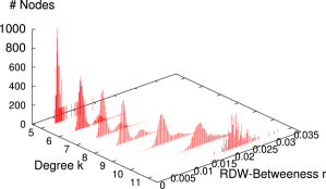
Figure 2: Correlation of degree and RDW betweenness for 100 SW-networks with $p=0.05$, $8$ nearest neighbors and $n=2000$ with corresponding RDW betweenness distribution.

For the Small-World model we have studied values $k=8,16,24$ and $p=0.05,0.10,0.15$. We observe usually moderately high correlations, but lower than for the ER model (not shown directly, see below). For the degree-RDW betweenness correlation, the data points are not uniformly distributed, similar to the betweenness-RDW betweenness we have shown for the ER graphs above. This can be seen here better when looking at the correlation using a three-dimensional plot of impulses, rather than a scatter plot, see Fig. 2. The ”‘oscillation”’ that can be observed is also consistently present in the overall distribution of the RDW betweenness (averaged over all degrees). Hence, here also two types of vertices seem to be present, but the distinction is weaker than above. Even for very small probabilities (i.e. $p=0.0001$, $n=2000$, $k=8$) the two peaks are visible though they are very close together. The gap between the two peaks gets larger the higher the rewiring probability $p$. Here, the difference seems to be strongly related to the re-wiring of the nodes, because for the case $k=8$, i.e. the degree of the corresponding $p=0$ network, the two peaks in the distributions are most clearly separated.

Figure 3: A SW-network with ten nodes. The numbers indicate the random-walk betweenness of a node. The node with a newly gained edge by rewiring obtains a much higher value than the others, while the node which lost an edge obtains a much lower value.

Even for very small network sizes like 20 nodes, it is possible to see two different peaks. Consider for example the 20 node network shown in Fig. 3, where just one edge has been rewired. The node with the highest value for the random-walk betweenness is the one that gained an additional edge by re-wiring. It is also visible that nodes with the same degree get different values for the RDW-Betweenness, which become smaller with growing distance to the most important node. This explains why the peaks get smeared out: It is because the nodes that get new edges influence those nodes that stay the same from a degree point of view. In general even nodes that keep their degree constant but gain crosslinks to high RDW betweenness nodes get a similarly high RDW betweenness. So one explanation of the peaks would be that the lower peak is a smeared out version of the one-value peak before rewiring and the the peak for higher RDW betweenness values appears because rewired nodes get a much higher RDW betweenness.

Figure 4: Correlation of degree and RDW betweenness for 100 BA networks with $m=8$ and $n=2000$.

The Barabási-Albert networks, where we have studied values $m\in{8,16,24}$, show again almost linear correlations for all combinations of measures. Nevertheless, the correlations were not as clear as for the Erdő-Rényi networks, i.e. we observed a much larger scattering of the data, but in the same order of magnitude as for the SW graphs. An example can be seen in Fig. 4. Here, we did not observe any particular strange correlation for any combination of measures, in contrast to the other two models.

Hence, to summarize the study of the correlations for the random graphs (results for the distributions, in particular exponents in case of power-law behavior, see below), we find most of the time a strong correlation between all different centrality measures, hence the degree is almost sufficient to characterize the importance of a node. This statement is certainly not true for many networks based on real-world data, as we will see next.

Figure 5: Correlation of betweenness and RDW betweenness for the AS network.

The AS network exhibits a positive correlation for all combinations of measures. Nevertheless, the results show some aspects of the behavior which is strongly different from the networks models discussed previously. E.g.  a scatter plot of betweenness against RDW betweenness is shown in Fig. 5. One can see that the scatter of the data points appears is always very small. This indicates that the fluctuations generated by the local structure around a node are always of the same order of magnitude, irrespectively of the absolute value of a quantity. Furthermore, even more interestingly, we observe that almost all data points obey the inequality $r\geq b$. So far we do not have an explanation for this effect, which is not present in the data for the network models.

(a) The PIN-network.

(b) A BA network with similar degree-distribution.

Figure 6: Comparison of degree-SC correlation between BA-Model and PIN-network

The calculations on the PIN network presented high correlations on all combinations of measures (not shown) except the degree-SC correlation plot, see Fig. 6(a). Here you can see two ”‘branches”’ that contain the data points. Thus, there are two types of vertices. For one type, the number of closed walks increases exponentially with the degree. This is the behavior, we have for complete (sub-) graphs (cliques), i.e. where each protein interacts with each other member of the (sub-) graph. On the other hand, there are proteins, where the participation in closed walks does not increase at all with the degree, which means that these proteins, although possibly with a large number of interacting partners, participate nevertheless only loosely in the overall interaction network. Note that for large degrees, there seem to be even proteins, which interpolate between the two limiting behaviors. This behavior is quite the different to what you find with for example for the BA networks and it is a hint that the structure of this network cannot be modeled with BA networks although it degree distribution, which we have measured as well (see below), is still scale-free. To illustrate this we tried to fit a BA network’s degree distribution as good as possible to the degree distribution of the PIN network and found the best fit for $m=2$ and $k_{0}=-1$, although the BA networks for these parameters have generally a smaller maximum degree than the PIN network. As you can see in Fig. 6(b) the correlation plots look completely different. For different values of $m$ and $k_{0}$ the scales of the axes change (especially the SC yields much higher values in the same order of magnitude as the PIN network) but the generally behavior is consistent. A model for such an interaction network would have to take the existence of two types of proteins into account, resulting in two different rules for the creation of the nodes. In a recent study of the PIN network pinsc which also uses a few centrality measures it is found that high subgraph centrality is a better hint for essential proteins than for example the degree. Thus it fits nicely to our result that the degree and subgraph centrality are not strongly correlated in this case.

Figure 7: Correlation of degree and RDW betweenness for the GEOM network.

Figure 8: Correlation of betweenness and RDW betweenness for the GEOM network.

For the GEOM network the measure1-measure2 correlation plots show a quite scattered behaviour, i.e. much smaller correlations than seen in the network models, see e.g. Fig. 7. Here we also observe the $r\geq b$ feature in the betweenness-RDW betweenness correlation plot, see Fig. 8. but the effect is even stronger in comparison to Fig. 5. Hence, this inequality might be a property seen in many networks based on real-world data and it certainly deserves a more thorough investigation.

Figure 9: Correlations of betweenness and RDW betweenness on the ECOLI-network

For the ECOLI network, the correlations of the measures range from moderately correlated highly to highly correlated, see e.g. Fig. 9. In principle, the plots look quite similar to those of the AS network. Here we could not observe any particular new properties, hence we do not go into further details for this network type.

Name	Degree	Betweenness	RDW-Betweenness
AS	1.54(4)	1.66(3)	1.55(3)
GEOM	2.34(6)	1.86(5)	1.51(4)
ECOLI	2.87(9)	2.18(9)	3.1(1)
PIN	1.65(4)	1.82(4)	1.66(3)

Table 1: Power-Law Exponents

Finally, we look just at the distribution of the centrality measures for the real-world networks. We find that all the real networks show a scale-free behavior, see e.g. Fig. 10. We have fitted power laws $P(x)\propto x^{\gamma}$ to all data except for the the subgraph centrality, where the data was distributed only over a small interval, so a fit would be meaningless. The power-law exponents we calculated can be found in table 1. This shows that when just looking at the distributions of centrality measures, the behavior of the real-world network is also found for the BA model. Goh et al. Goh also found that for this model the betweeness distribution follows a power law. Only when considering correlations between different measures, one realizes that the so-far existing models, although having provided much value insight, have to be extended and/ or modified, to really capture the behavior found in the behavior of proteins, metabolic pathways, humans and other systems represented by networks.

Figure 10: RDW betweenness distribution for the GEOM network.

VI Conclusion

In this paper we have studied four different local and global centrality measures to analyze the behavior of different model and real-world networks. First, the choice which measure is “most suitable” depends on the network that is used and which kind of information shall be extracted by calculating that measure. There does not seem to be an overall best measure that is optimal for all applications. The shortest-path betweenness might be feasible if the network can be assumed to contain global knowledge of optimal routes. But even in this case, when much traffic is on the network, it is certainly very often advisable to use non-shortest paths to reach the destination as quick as possible. In cases where participation in social sub-groups is of interest the subgraph centrality might be best whereas in situations where each node only passes information randomly to its nearest neighbors the random-walk betweenness should be the method of choice.

Nevertheless, in order to understand really how a network is organized, it sees not to be sufficient to study just one measure and its distribution. We have seen that for all real-world networks considered here, the distributions of all measures is indeed well described by power laws. But when considering correlations between different centrality measures we see that the most common random network models reflect the truth only partially since the scatter plots do look quite different compared to the real networks.

It seems that network models have to be more specifically for each application. One single mechanism like preferential attachment, at least if being used as the only mechanism to create the graph, is too simple to explain the complex properties of real-world networks. Models that incorporate evolution and growth of networks as represented for example in NetworkEvo might be the key to give deeper insight why many networks show a scale-free behavior for one of their properties and still differ from simpler models like the BA model. Since each application will need its specific mechanism to generate a network, proposing new models for specific applications is beyond the scope of this work.

- (1) J. Scott, Social Network Analysis: A Handbook, (Sage, London, 2000).
- (2) Peter Holme and Beom Jun Kim, Attack vulnerability of complex networks, Phys. Rev. E 65, 056109 (2002)
- (3) D. Brockmann, L. Hufnagel and T. Geisel, The scaling laws of human travel, Nature 439, 462 (2006).
- (4) R. Albert and A.-L. Barabási, Statistical mechanics of complex networks, Rev. Mod. Phys. 74, 47 (2002).
- (5) M. E. J. Newman, The structure and function of complex networks, SIAM Review 45, 167 (2003).
- (6) A.-L. Barabási and R. Albert, Emergence of scaling in random networks, Science, 286, 509 (1999).
- (7) A.-L. Barabási, R. Albert, and H. Jeong, Mean-field theory for scale-free random networks, Phys. A, 272, 173 (1999).
- (8) L.C. Freeman, A set of measures of centrality based upon betweenness, Sociometry 40, 35 (1977).
- (9) M. E. J. Newman, A measure of betweenness centrality based on random walks, Social Networks 27, 39 (2005).
- (10) Ernesto Estrada and Juan A. Rodíguez-Velázquez, Subgraph centrality in complex networks, Phys. Rev. E 71, 056103 (2005).
- (11) L.C. Freeman, Centrality in social networks: Conceptual clarification, Social Networks 1, 215 (1979).
- (12) M. E. J. Newman, Scientific collaboration networks: II. Shortest paths, weighted networks, and centrality, Phys. Rev. E 64, 016132 (2001).
- (13) P. Erdős and A. Rényi On random graphs, Publ. Math. Debrecen 6, 290 (1959).
- (14) P. Erdős and A. Rényi On the evolution of random graphs, Magyar Tud. Akad. Mat. Kutató Int. Közl. 5, 17 (1960).
- (15) P. Erdős and A. Rényi On the strength of connectedness of a random graph, Acta Math. Acad. Sci. Hungar. 12, 261 (1961).
- (16) D. J. Watts, Networks, dynamics, and the small world phenomenon, Amer. J. Sociol. 105, 493 (1999).
- (17) D. J. Watts, Small Worlds, Princeton University Press (Princeton, NJ, 1999).
- (18) D. J. Watts and S. H. Strogatz, Collective dynamics of ”small-world” networks, Nature 393, 440 (1998).
- (19) Project COSIN http://www.cosin.org. For the AS network we used the data set from 2000/04/03.
- (20) Hongwu Ma and An-Ping Zeng Reconstruction of metabolic networks from genome data and analysis of their global structure for various organisms Bioinformatics Vol. 19 no. 2 (2003) Pages 270-277.
- (21) KEGG: Kyoto Encyclopedia of Genes and Genomes http://www.genome.jp/kegg/
- (22) Data for Computational Geometry by V. Batagelj http://vlado.fmf.uni-lj.si/pub/networks/data/
- (23) Lloyd Demetrius and Thomas Manke Robustness and network evolution - an entropic principle Physica A 346 (2005) 682-696.
- (24) B. Bollobás, O. Riordan, J. Spencer, and G. Tusnády, The degree sequence of a scale-free random graph process, Random Structures Algorithms, 18 (2001), pp. 279-290.
- (25) K.-I. Goh, B. Kahng, D. Kim, Phys. Rev. Lett. 87, 278701 (2001)
- (26) Ernesto Estrada, Virtual identification of essential proteins within the protein interaction network of yeast, Proteomics 6: pp. 35-40 (2006)
- (27) The Internet Movie Database http://www.imdb.com.