Computational Euler History

Abstract

A new pseudospectral calculation of collapsing Euler vortices Hou & Li (2006) has called into question the long-term conclusions of singular behavior described earlier in Kerr (1993, 2005). This review is designed to: improve the discussion of the detailed analysis of one test initial condition designed find sources of errors, to compare that with calculations showing no evidence of a singularity, and to document two sets of discussions. Those prior to 1993 between competing teams. And recent discussions of what is needed to reach more convincing conclusions.

1 Introduction

Whether or not there are singularities of the incompressible three-dimensional Euler equations is of fundamental mathematical and physical importance. This review will not discuss either of these issues or related questions for how this behavior could be applied to our understanding of partial differential equations or turbulence theory. Instead, the focus will be the history, circa 1990, of numerical calculations that were designed to determine if there could be a singularity of the three-dimensional incompressible Euler equations and how, through several workshops, a concensus was reached about to address the issue numerically. Analytic results will not be discussed other than how they pertain to these calculations. One test calculation from Kerr (1992) will be used to suggest that the differences between the structures in the new calculation by Hou & Li (2006) and those presented by Kerr (1993) could be associated with small-scale noise. How this could disrupt a singular structure forming is discussed.

The paper is organized as follows. After the early history of Euler calculations is given, methodologies agreed upon by concensus at several workshops are presented, including how to compare calculations. Next is a discussion of the uses and dangers of the most robust approach, namely pseudospectral methods. Then a section compares Kerr (1993) to competitive calculations from the early 1990s. Finally there is a comparison between Kerr (1993) and Hou & Li (2006).

2 Early Euler calculations

The first serious attempt to study Euler numerically was the Taylor-Green calculations of Brachet et al. (1983). Their conclusion was that vortex sheets suppressed any trends towards singularities that had previously been suggested either by spectral closures or series expansions. This conclusion was qualitatively similar to the conclusion from two-dimensional ideal, incompressible MHD calculations (Sulem et al. (1985)) where it was found that current sheets suppressed trends towards singularities.

The next set of numerical investigations used vortex filaments. While these are a poor approximation of the Euler equations at the smallest scales, they did provide a global picture that an anti-parallel initial condition might predispose a calculation towards singular behavior in a manner that smooth initial conditions might not (Pumir & Siggia (1987)). This led to two preliminary studies at low resolution (Ashurst & Meiron (1987); Pumir & Kerr (1987)) whose only significant contribution was that vortex flattening might play a role similar to current sheets in 2D MHD. Simultaneously, an orthogonal initial condition was simulated that showed more curvature development than the anti-parallel simulations (preliminary results by Melander and Zabusky in 1988 eventually appeared in Boratav et al. (1992)).

All the subsequent calculations assumed an anti-parallel geometry, for which there are two symmetry planes. One in $y-z$ is between the vortices and was called the ‘dividing plane’. The other in $x-z$ is at the position of maximum perturbation and was called the ‘symmetry plane’. (Terminology due to F. Hussain.) The next step was to find a better initial condition within this geometry and the first steps towards adaptivity. Melander & Hussain (1989) were able to identify an initial condition where all derivatives in the profile of the vortex core went smoothly to zero and used a sinusoidal perturbation of the $x-z$ position as a function of $y$. The calculation did not take advantage of the symmetries, had uniform mesh spacing in all direction and was viscous. Kerr & Hussain (1989) tried a truncated Gaussian core and resolved the discontinuities at the edge of the initial condition by applying a strong Fourier based hyper-viscous filter. Kerr & Hussain (1989) used a combination of higher order trigonometric functions to create an initial perturbation that was localized near the symmetry plane. Symmetries were used to reduce the computational requirements, the mesh spacing depended upon direction and the calculations were viscous. Pumir & Siggia (1990) uses a hyperbolic trajectory for the vortex lines, therefore being the only calculation to date that is not in a periodic geometry. They used a strictly Gaussian core that does not ever go to zero, which is possible if one does not have to worry about overlapping across periodic boundaries. Their calculation was completely adaptive and inviscid.

Of these calculations, only the viscous calculation of Kerr & Hussain (1989) had any consistency with singular behavior. To test the Melander & Hussain (1989) profile in adaptive calculations, Kerr (1993) and Shelley et al. (1993) tried Chebyshev and mapped Fourier methods respectively. Kerr (1993) reported consistency with the singular trends of Kerr & Hussain (1989). Shelley et al. (1993) concluded that the trends did not favor a singularity, but their calculations used only the sinusoidal perturbation of Melander & Hussain (1989) and were viscous. Why they reached different conclusions was discussed briefly by Kerr (1992) and will be discussed further here in subsection 5.3.

The only significant calculations since then are due to Grauer et al. (1998) and now Hou & Li (2006). The Grauer et al. (1998) calculation seems consistent with the trends in Kerr (1993) while Hou & Li (2006) is not. Kerr (1993) and Hou & Li (2006) are compared in section 6. The Kida vortex promoted by Pelz (2001) as a scenario for a singularity has recently been shown to be regular by Grauer (private communication).

3 Workshop methodologies

The methodology of Pumir & Siggia (1990) and Kerr (1993) was worked out at two workshops on Topological Fluid Dynamics chaired by H. K. Moffatt in 1989 and 1991. These were the IUTAM Symposium on Topological Fluid Dynamics in August 1989 in Cambridge, England and the Program on Topological Fluid Dynamics at the Institute for Theoretical Physics in Santa Barbara in the Fall of 1991, with a symposium on issues in Euler at the end of October 1991.

The following principles were worked out at those programs in discussions between most of the principal authors at that time such as U. Frisch, F. Hussain, R.M. Kerr, R. Pelz, A. Pumir E.D. Siggia, N. Zabusky, and the other participants in those workshops.

These are some of the rules:

1. Run only Euler. Do not try to reach conclusions about Euler using a series of decreasing viscosity Navier-Stokes calculations. The range of Reynolds numbers available to Navier-Stokes calculations at that time is too short to be useful in reaching any definite conclusions.

2. Use refined meshes. Even the easy solution of different mesh sizes in different directions, as in Kerr & Hussain (1989), has limitations. There is too much space over which nothing is happening. Complementary pseudo-spectral calculations can still be useful to confirm the numerical method, but serious compromises have to be made as discussed below.

3. Have a localized initial perturbation. Orthogonal vortices and the hyperbolic trajectory of Pumir & Siggia (1990) automatically satisfy this. Kerr & Hussain (1989) and Kerr (1993) satisfy this condition using a map of a sinusoidal perturbation.

4. One needs to demonstrate structures that wouldn’t be subject to depletion of nonlinearity. In particular if vortex sheets appear, they must develop strong curvature or kinks.

5. The primary quantity of interest is the $L_{\infty}$ norm of vorticity $\|\mbox{\boldmath$\omega$}\|_{\infty}~{}$ so that consistency with the analytic result of Beale et al. (1984) can be tested. If singular behavior is suspected, then the following must be obeyed:

   $$\int_{0}^{t}\mbox{$\|\mbox{\boldmath$\omega$}\|_{\infty}~{}$}dt\rightarrow\infty$$ (1)

6. If it has power-law behavior of the form $\mbox{$\|\mbox{\boldmath$\omega$}\|_{\infty}~{}$}\sim(T-t)^{-\gamma}$ and $\gamma<1$, then the calculation is incorrect.

7. The best way to test (1) is to assume $\gamma=1$. This would be dimensionally consistent.

8. However, using $\|\mbox{\boldmath$\omega$}\|_{\infty}~{}$by itself can lead to misleading conclusions either way. Double exponentials are indistinguishable from power laws and at late times it is impossible to avoid some slowing of singular trends, which could lead to the appearance of saturation if one assumes that $\alpha=d\mbox{$\|\mbox{\boldmath$\omega$}\|_{\infty}~{}$}/dt$.

9. Therefore one must calculate the time derivative of $\|\mbox{\boldmath$\omega$}\|_{\infty}~{}$directly, that is $\alpha=\omega_{i}e_{ij}\omega_{j}/|\omega|^{2}$ directly, which should also have time-integral singular growth (Ponce (1985)). In the anti-parallel case $\alpha$ is just the velocity derivative on the symmetry plane of the axial velocity. This gives an independent measure of singular activity While finding $\alpha_{p}$ at the point of $\|\mbox{\boldmath$\omega$}\|_{\infty}~{}$ is most desirable, finding $\alpha_{s}=\sup(\alpha)$ in the symmetry plane was found to work better in Kerr (1993).

10. One needs a measure of collapse to satisfy the condition of Caffarelle et al. (1982).

Some of these rules were refined by further conversations between R.M. Kerr and A. Majda during a two week workshop at the Research Institute in Mathematical Sciences in Kyoto, Japan in October 1992.

Besides the rules just listed, other tests that have been tried and their order of success are as follows:

• Finding independently that

  $$\Omega_{pr}=\int dV\omega_{i}e_{ij}\omega_{j}\sim\frac{1}{T-t}$$ (2)

  with the same singular time as for $\|\mbox{\boldmath$\omega$}\|_{\infty}~{}$and $\alpha$. The evidence from Kerr (1993) is that this test works better than finding either $\alpha_{p}$ or $\alpha_{s}$ defined above.

• Pumir & Siggia (1990) discusses how the position of $\|\mbox{\boldmath$\omega$}\|_{\infty}~{}$moves. Kerr (1993) goes further and tries to show that the positions $(x,z)_{p}$ of all minima and maxima of components of the stress tensor in the symmetry plane collapse to the positions of $\|\mbox{\boldmath$\omega$}\|_{\infty}~{}$. That is

  $$x_{p}-X(T)\sim T-t\quad,\quad z_{p}\sim T-t$$

• Kerr (2005) goes further still by looking at profiles.

• $\sup(|v|^{2})\sim T-t$ where $v$ is the axial velocity in the direction of vorticity in the symmetry plane. This would provide consistency with a suggestion from Constantin et al. (1996). The only evidence for this is marginal from Kerr (2005). We need a good calculation to test this.

• Curvature blowup as $\kappa^{-2}\sim(T-t)$. Again, this would provide consistency with a suggestion from Constantin et al. (1996). So far this is only inferred by related scaling properties in Kerr (2005). Again, a good calculation is needed to test this.

4 Uses and pitfalls for pseudospectral

For any problem where most of the domain is not involved in the dynamics, as for this possibly singular equation, uniform mesh methods waste most of the computational domain. Pseudospectral codes fall into this class of methods. Besides being limited in the local resolution they can provide, pseudospectral codes have the additional annoyance of a continuing debate over how to handle the high wavenumber cutoff.

Many strategies have been tried over the years. Initially Orszag and Patterson decided upon a spherical truncation which was corrected by adding together two phase-shifted versions of the nonlinear terms. Then NASA Ames proposed the Leonard filter for LES calculations. By the mid-1980s it was generally agreed that none of these tricks gained one anything. LES calculations started using only a sharp-wavenumber cutoff with the 2/3rds rule and DNS in wall-bounded flows at NASA Ames/CTR did the same. All of my calculations after 1985, whether Euler, Navier-Stokes, or convection have followed this policy.

The issue has been reopened by Hou & Li (2006) claiming to have found a filter with 36th-order accuracy. So let me summarize my understanding of the good and bad points of different methods for the Euler problem.

Options for high wavenumber cutoff of Euler:

• 2/3rds dealiasing.

  • Good: absolutely no wavenumber contributions for $k>(2/3)k_{max}$, which would immediately give errors.

  • Good: energy is exactly conserved.

  • Bad: An abrupt cutoff leads to Gibbs phenomena (oscillations) in physical space.

  • Solution: Must set a strict standard when the calculations must be shut off based upon anomalous growth of the wavenumbers near the cutoff. This is good in that there is a measure of the errors.

• A smooth filter that ends for $k=(2/3)k_{max}$.

  • Good: minimize Gibbs phenomena.

  • Bad: Dissipative.

  • Bad: No measure of errors.

• A smooth filter that extends beyond $k=(2/3)k_{max}$.

  • Good: Maybe minimizes Gibbs phenomena.

  • Bad: Immediately adds aliasing errors.

  • Bad: might add small regions of negative vorticity that can blow up.

  • Bad: No measure of errors.

  • Unsolved: What of the claim in Hou & Li (2006) that this converges? And how does one identify what the aliasing errors turn into?

Despite these problems, it was concluded that in the early stages a pseudo-spectral code is much better for testing initial conditions, in particular testing schemes for filtering the initial condition. It was in ensuring that the nonlinearity was not depleted even at low resolution and early times in such test calculations that led to the initial condition and numerics that worked so well in Kerr (1993).

Figure 1: $\|\mbox{\boldmath$\omega$}\|_{\infty}~{}$ and $\alpha$ contours in the symmetry plane for $t=15$ from Kerr (1993)

Figure 2: Dependence of $1/\mbox{$\|\mbox{\boldmath$\omega$}\|_{\infty}~{}$}$, $0.1/|e_{yy,p}|$ and $0.0003/\Omega_{pr}$ upon time from the anti-parallel Euler calculation showing convergence to a singular time of about $T=18.7$.

Figure 3: Initial $z$-Chebyshev distribution (spectrum) for filtered intial conditions.

Figure 4: Dependence of $\|\mbox{\boldmath$\omega$}\|_{\infty}~{}$, $|e_{yy,p}|^{-1}$ and $|e_{yy,p}|$ upon time from the filtered initial condition anti-parallel Euler calculation

Figure 5: $\omega$ in the symmetry plane, $z$ is not stretched, for $t=0$, 6, 12 and 15.5

5 Comparison of structures and $\|\mbox{\boldmath$\omega$}\|_{\infty}~{}$between older calculations

This section will compare three calculations that meet the simulation criteria (a-c) above:

• Kerr (1993)

• An intermediate time from Pumir & Siggia (1990).

• An inviscid version of the Shelley et al. (1993) calculation.

Earlier calculations such as Ashurst & Meiron (1987), Pumir & Kerr (1987) and Melander & Hussain (1989) met none of these criteria on coarse meshes.

When Kerr (1993) was published, the weight of numerical evidence from simulations with similar initial conditions was against a singularity. Therefore, in making claims of singular behavior, besides demonstrating points (a-k) above,the following was addressed:

• The computational power of the calculations finding exponential growth was matched.

• A modification of the singular initial condition was found that was able to reproduce the exponential behavior of competitive calculations.

• A proposal was made for why there could be at least two types of behavior, exponential and singular.

While Pumir & Siggia (1990) and Kerr (1993) meet all three requirements, the published work of Shelley et al. (1993) was neither inviscid nor did it have a localized perturbation. A better description of Shelley et al. (1993) is that it was a slightly adaptive and higher Reynolds number version of Melander & Hussain (1989). Nonetheless, by giving the profile they used a localized perturbation and running it inviscidly, the primary conclusion of Shelley et al. (1993) could be verified. This was that for the Melander & Hussain (1989) profile, singular behavior does not appear.

The goal of working by steps through these three cases is to suggest how the calculation of Hou & Li (2006) might be suppressing singular behavior due to numerical noise in their numerical method. The first step follows Kerr (1992) to show how the initial condition of Shelley et al. (1993) leads to false regular behavior. Then the graphics for an inviscid version of Shelley et al. (1993) is compared to the very late times of Pumir & Siggia (1990). In this way the structures associated with regular behavior will be identified. Finally, similar structures are identified in Hou & Li (2006). This raises the possibility that the numerical method of Hou & Li (2006) also introduces small scale numerical errors. This will only be confirmed if their 2/3rds dealiasing calculations are report or are repeated by someone else.

Figure 6: $\|\mbox{\boldmath$\omega$}\|_{\infty}~{}$ and $\alpha$ contours in the symmetry plane for $t=7.2$ from Pumir & Siggia (1990)

Figure 7: Growth of $\|\mbox{\boldmath$\omega$}\|_{\infty}~{}$, $\alpha$ from Pumir & Siggia (1990)

5.1 Comparing structures of Kerr (1993) and Pumir & Siggia (1990)

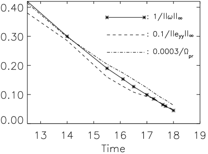
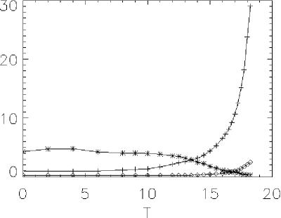
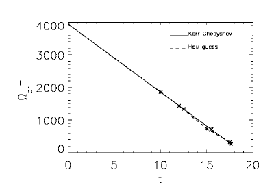
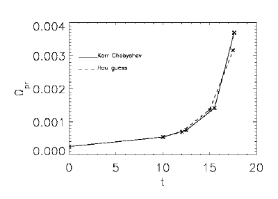
The purpose of this subsection is to compare the structures that arise during the period with the strongest evidence for singular growth of Kerr (1993) with a brief period of growth from Pumir & Siggia (1990) that might have consistent behavior. Figure 2 from Kerr (2005) shows the growth of $\|\mbox{\boldmath$\omega$}\|_{\infty}~{}$, max($\alpha$)=$\|e_{yy}\|$ in the symmetry plane, and the enstrophy production $\Omega_{\rm pr}$. This was the primary evidence that these calculations have singular growth. Figure 4 plots the peak vorticity, peak strain along the vorticity in the symmetry plane, and the inverse of that strain as functions of time for a $256\times 256\times 192$ pseudospectral calculation using the initial condition of Kerr (1993). This pseudospectral calculation was not the best that was done in preparation for the final calculations of Kerr (1993), but it can be used to illustrate the differences between this initial condition and the Melander & Hussain (1989) initial condition. The peak of the $\alpha_{\infty}=\|e_{yy}\|_{\infty}$ strain is plotted instead of the value at the position of $\|\mbox{\boldmath$\omega$}\|_{\infty}~{}$ because it was better behaved as previously discussed (Kerr (1993)).

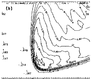
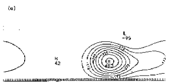
The vorticity and strain contours in Fig. 2 are straight out of Kerr (1993) for $t=15$. These plots have been expanded by a factor of 5 in the vertical ($z$) direction. This time was chosen because it shows the least numerical noise while being the regime showing singular growth of $\|\mbox{\boldmath$\omega$}\|_{\infty}~{}$. Subsequent to 1993 it was realized that most of the noise in the contours in Kerr (1993) comes from a high wavenumber spectral tail, which when filtered out gives the smoother figures of Kerr (2005). It is likely that the physical space data for these fields in this plane is still stored on the NCAR mass store and might be used later to create better figures.

The two points of comparison to be made are that:

1. The highest contour of vorticity is placed in the corner of the bent front.

2. There is a steepening of the positive strain contours in the direction of propagation of the front.

To compare with competitive calculations whose graphic results do not stretch the inter-vortical ($z$) direction, it is useful to show contour plots of vorticity in the symmetry plane without stretching in Fig. 5. The evolution with time is as follows:

• At $t=6$ there is only flattening.

• At $t=12$ a tilt in the innermost contour appears.

• This becomes more of a crescent in the bend at $t=15.5$, which is essentially an unstretched version of left frame of Fig. 2 with the highest vorticity contour only within the bend.

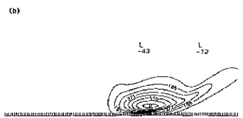
How does this compare to Pumir & Siggia (1990)? Recall that they use hyperbolic trajectories, while all the other calculations use periodic trajectories. Therefore, definitive comparisons are out of the question. Nonetheless, Fig. 7 shows that growth of $\|\mbox{\boldmath$\omega$}\|_{\infty}~{}$ and $\alpha_{p}$, the strain at the position of $\|\mbox{\boldmath$\omega$}\|_{\infty}~{}$, in Pumir & Siggia (1990) is similar to Fig. 2. Recall that in Kerr (1993) it was found that while $\|e_{yy}\|_{\infty}\approx 0.1\mbox{$\|\mbox{\boldmath$\omega$}\|_{\infty}~{}$}$, $\alpha_{p}\approx 0.05\mbox{$\|\mbox{\boldmath$\omega$}\|_{\infty}~{}$}$. Therefore there is a short period between $t=7.6$ and $t=8.1$ where the growth of $\|\mbox{\boldmath$\omega$}\|_{\infty}~{}$ and $\alpha_{p}$ in Pumir & Siggia (1990) might be consistent with Kerr (1993). Most of the growth of $\|\mbox{\boldmath$\omega$}\|_{\infty}~{}$ before $t=7.6$ is just to set up the structure. $t>8.1$, when saturation appears, is discussed in the next subsection.

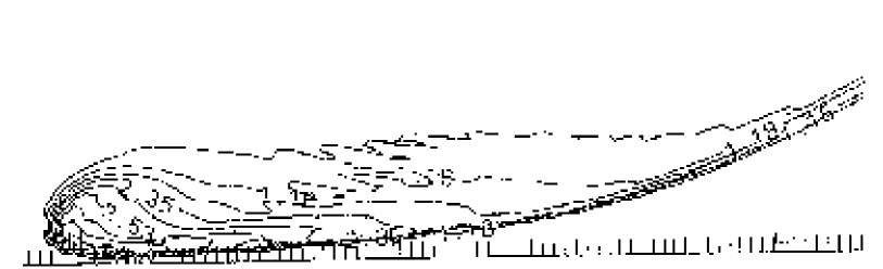
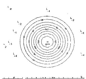
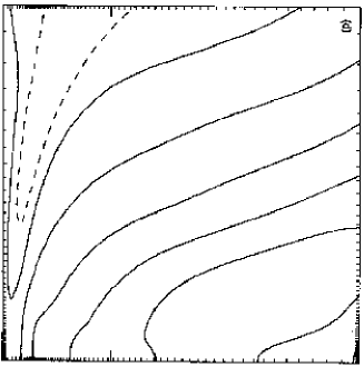
Figure 7 shows contours of $\|\mbox{\boldmath$\omega$}\|_{\infty}~{}$ and $\alpha$ just before this period at $t=7.2$. As in Fig. 2, the highest contour of vorticity is placed in the corner of the bent front and there is a steepening of the positive strain contours in the direction of propagation of the front. There is a long tail in the vorticity plot, but it seems to be separating from the contour in the corner. In these respects the figures are similar to Kerr (1993).

The next subsection will show that when non-singular growth is observed, these properties are not observed.

5.2 Initial profile and why a localized perturbation with filtering is used

There are two critical components in forming the initial condition previously discussed by Kerr (1992) and Kerr (1993).

• First is using a vortex core profile that, before smoothing, is analytic as originally proposed by Melander & Hussain (1989). As they claimed, their profile is far superior to the cut-off Gaussian profile used by Kerr & Hussain (1989). However, even here, based on spectra (see below), it was decided that this it was not smooth enough and a small high-wavenumber filter was necessary.

• Second, there is the intertwined choices of the initial perturbation in the trajectory of the vortex tube and of the dimensions of the periodic domain in the axial direction. This is discussed next.

Following Kerr & Hussain (1989) the trajectory of the center of the initial vortex tubes was defined as

$$X(s)={x_{\circ}}+{\delta_{x}}\cos(s)$$

$$Z(s)={z_{\circ}}+{\delta_{z}}\cos(s),\quad\rm{where}$$

$$s(Y)={y_{2}}+{L_{y}}{\delta_{y1}}\sin(\pi{y_{2}}/{L_{y}})\quad\rm{and}$$

$${y_{2}}=Y+{L_{y}}{\delta_{y2}}\sin(\pi Y/{L_{y}})$$

rather than a simple sinusoidal trajectory.

The incompressible vorticity vector for this trajectory was proportional to

$$\begin{array}[]{rcl}\omega_{x}&=&-\dfrac{\pi\delta_{x}}{L_{y}}\left[1+\pi\delta_{y2}\cos\left(\dfrac{\pi y}{L_{y}}\right)\right]\times\left[1+\pi\delta_{y1}\cos\left(\dfrac{\pi y_{2}}{L_{y}}\right)\right]\sin\left(\dfrac{\pi s(y)}{L_{y}}\right)\\ \omega_{y}&=&1\\ \omega_{z}&=&-\dfrac{\pi\delta_{z}}{L_{y}}\left[1+\pi\delta_{y2}\cos\left(\dfrac{\pi y}{L_{y}}\right)\right]\times\left[1+\pi\delta_{y1}\cos\left(\dfrac{\pi y_{2}}{L_{y}}\right)\right]\sin\left(\dfrac{\pi s(y)}{L_{y}}\right)\end{array}$$

Following a suggestion by Melander (private communication) the profile of vorticity about this trajectory was given by

$$\omega(r)=\exp(f(r)),$$

where

$$f(r)=-\frac{r^{2}}{1-r^{2}}+r^{2}(1+r^{2}+r^{4})$$

and a distance $r$ from the center of the vortex core $(X,Y,Z)$ of characteristic radius $R$ is

$$r=|(x,y,z)-(X,Y,Z)|/R\quad\rm{for}\quad r\leq 1$$

These formulae have been corrected based upon errors in the text of Kerr (1993) noted by Hou & Li (2006). Hou & Li (2006) missed the following additional misprint. In Kerr (1993) and Hou & Li (2006) in the formulae for $X(s)$ and $Z(s)$ (or their equivalents) , ’$/L_{x}$’ and ’$/L_{z}$’ respectively should both be ’$/L_{y}$’.

For $\delta_{y1}=\delta_{y2}=0$ the trajectory is sinusoidal, as used by Melander & Hussain (1989). Two problems were then identified with the procedure of Melander & Hussain (1989), which were replicated by Shelley et al. (1993).

The first problem identified by Kerr & Hussain (1989) was that if a sinusoidal perturbation is used then, as the two vortices collapse in the direction between themselves, they also expanded in the axial $y$ direction. When this expansion runs into its periodic image, growth in $\|\mbox{\boldmath$\omega$}\|_{\infty}~{}$ is suppressed. Doubling the domain size in $y$ does not resolve the problem. Therefore to localize the perturbation, Kerr & Hussain (1989) and Kerr (1993) chose the following values of $\delta$: $\delta_{y1}=0.5,\delta_{y2}=0.4,\delta_{x}=-1.6$and $\delta_{z}=0$ and $z_{\circ}=1.57$ and $R=0.75$.

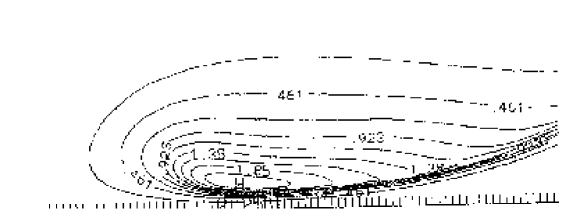
A more serious problem was that the initial profile of Melander & Hussain (1989), without any filtering, created regions of negative vorticity in the symmetry plane. There are small negative regions that cannot be seen in the contour plots unless either zero contours are plotted or highs and lows are given. This is demonstrated in the first frame of Fig. 8.

When highs and lows as in Fig 8 are not used in the graphics, one cannot assess the possible impact of small negative regions. This would apply to the graphics in Pumir & Siggia (1990), Shelley et al. (1993) and now Hou & Li (2006) In Hou & Li (2006) negative contours would not appear in the initial condition because their initial condition is filtered, but evidence for negative regions at late times is discussed in the next section.

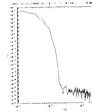
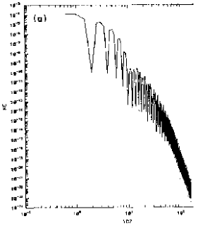
In preparation for the calculation in Kerr (1993) that used a filtered initial condition, a variety of initial conditions without filtering were experimented with. A common feature of all the initial $z$ spectra, or equivalently the initial distribution of Chebyshev polynomials, was that they went to zero with increasing wavenumber in a sawtooth power law fashion. An example spectrum is shown in Fig. 10. The envelope of the high wavenumber sawtooth approximately obeys $k^{-2}$.

If behavior where an exponential high wavenumber tail or a power law $k^{-\gamma}$ with $\gamma>2$ is to be allowed, this type of initial condition should not be used. In fact, Kerr (1993) found that $\gamma>3$ and associated $\gamma\rightarrow 3$ as the possible singular time was approached with the test that $\Omega_{pr}\sim 1/(T-t)$ 2.

Figure 8: $y$ vorticity perpendicular in the symmetry plane. $t=0$, $t=9$ and $t=13$ for Kerr (1993) calculation.

Figure 9: $z$-spectra for unfiltered initial conditions.

Figure 10: Peak strain along the vorticity (triangle), peak vorticity (circle), peak negative vorticity (plus) for unfiltered initial conditions vs. time.

Increasing the resolution used with the unfiltered initial conditions did not alter either the low wavenumber components of the spectra or the magnitude of the regions of negative vorticity. That is, regions of negative vorticity in roughly the same location and of the same magnitude appear. This type of spectral behavior is reminiscent of Gibbs phenomena, that is high wavenumber oscillations that occur when a Galerkin method tries to represent physical space discontinuities. This suggests that the origin of the sawtooth spectra and negative regions of vorticity is the sharp cutoff in the vorticity profile used by Melander & Hussain (1989), although possible inconsistencies between the initial perturbation and periodic boundary conditions might also have an influence. This is despite the analytic formula where all derivatives smoothly went to zero at the edge of the vortex tube. While this might work analytically, all that a numerical calculation sees is that the vorticity goes from a finite value on one side of a boundary to continuously zero on the other side.

5.3 Effect when there is no initial filter

The calculation in this section is meant to show that if the high wavenumber filter is not applied to the initial conditions, then the strain saturates, afterwhich the growth of the peak vorticity is exponential. Qualitatively everything about this calculation is the same as the initialization used by Kerr (1993). The only significant difference was that the high wavenumber hyperviscous filter was not used.

Only enough resolution to demonstrate these points was used. There are some weak signs that at the last time calculated that the strain is beginning to increase and singular behavior might be starting. However, given the success of the filtered initial conditions there did not seem to be any reason to follow this further.

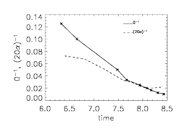
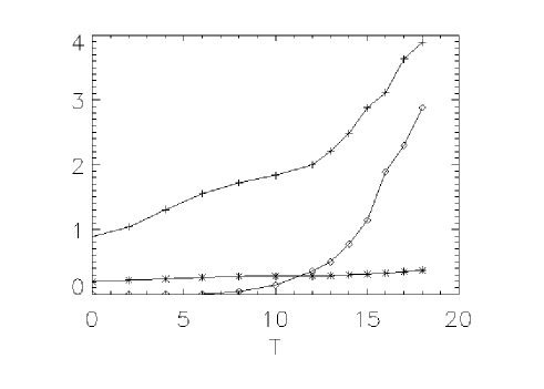
The suggestion at the end of the last subsection is that isolated points of negative vorticity might cause a problem. The best evidence that these negative regions do affect the calculation is that while they were initially very small, the order of $4\times 10^{-3}$ compared to the initial peak vorticity of 1, by the end of the calculation the negative peak was the same order of magnitude as the primary vortex. This is shown in Fig. 10.

Figure 10 also shows the strain, which saturates, leading to exponential growth of peak vorticity. It was also found that the position of the peak of $\alpha$ is the same distance from the dividing plane (in $z$) as the peak vorticity, whereas Kerr (1993) found that the strain peak is always somewhat further from the dividing plane.

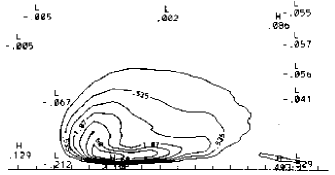
What are the differences in the structure? The second frame at $t=9$ shows that the vorticity that develops from initial condition Fig. 8 is not significantly different than the initial flattening from Kerr (1993), except it is remaining flat longer. At the slightly later time of $t=13$, a head-tail structure is found as in earlier viscous calculations of vortex reconnection. The difference with Kerr (1993) is that the highest contour is spread across a vortex sheet above the lower dividing plane, across from its mirror image.

The spreading of this innermost contour is the best indication that similar behavior might be happening in other calculations.

How might these negative regions create this change in structure? Detailed investigation of contours in preparing Kerr (1992) showed that the largest negative regions had been sucked into the region between the primary vortices, that is along the dividing plane. They then grow enormously and pair with their opposite number across the lower dividing plane and induce velocity opposite to that from the primary vorticity. This pulls the tail out and creates more flattening.

Figure 11: $\|\mbox{\boldmath$\omega$}\|_{\infty}~{}$ and $\alpha$ contours in the symmetry plane for $t=8.3$ from Pumir & Siggia (1990).

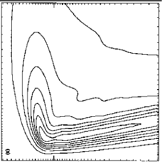
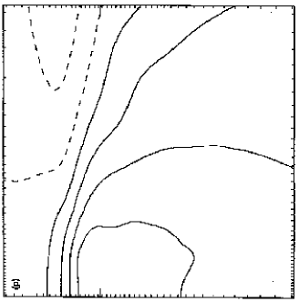
A comparison with the late times from Pumir & Siggia (1990) is now useful. That is for $t>8.1$, beyond when $\alpha_{p}\sim 0.05\mbox{$\|\mbox{\boldmath$\omega$}\|_{\infty}~{}$}$. Recall that in Fig 7, the strain was also observed to saturate at late times, with exponential growth of the peak vorticity. Based on these comparisons, the late times of Pumir & Siggia (1990) should be checked to see if there are similar regions of negative vorticity playing a major role, and if so to determine whether these regions might then explain the saturation of the strain in their calculations. The highest vorticity contour is now spread over the entire tail and the strain contours are not as concentrated.

Figure 12: Three-dimensional isosurface plot of the vorticity squared for $(x,y,z)=(4.9:8.8,0:3.9,0:3.9)$ at $t=12$ for unfiltered initial conditions.

Figure 13: Three-dimensional isosurface plot of the vorticity squared at $t=12$ for the filtered initial conditions in Kerr (1993).

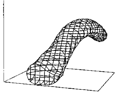
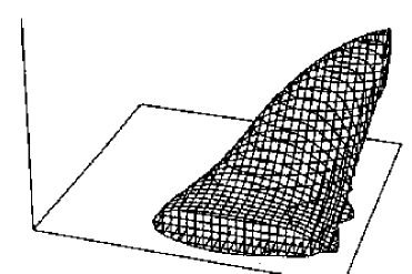
Figure 13 shows a three-dimensional isosurface plot of the vorticity squared at $t=12$ for the unfiltered initial condition and Fig. 13 an isosurface for the filtered initial condition at $t=12$. Overall, the three-dimensional structure for the unfiltered initial condition does not have two-dimensionalization of the vortices, one of the properties observed by Pumir & Siggia (1990), but does show less deformation than the filtered case from Kerr (1993). For the filtered initial condition, a crease in Fig. 13 where the isosurface moves away from the dividing plane indicates where three-dimensional curvature of the vortex lines is occurring. A similar crease does not appear for the unfiltered case.

Figure 14: Contour plots through the symmetry plane from Hou & Li (2006) at $t=15$ and 17 (left and right) with the same factor of 5 expansion in the vertical $z$ direction. The $t=17$ frame has been blown up by a factor of 6. Unlike Fig. 2, the $t=15$ contours here look more like the $t=6$ contours in Fig 5. Or $t=12$, except there is no upward tilt on the left, even some downward tilt. $t=17$ is very similar to the calculation with initial noise in Fig. 5

Figure 15: Comparison of enstrophy and enstrophy production between Hou & Li (2006) and Kerr (1993) assuming that they have the same values at $t=10$. The last two frames are $\Omega_{pr}$ not $\Omega$ as indicated. In Hou & Li (2006) the growth of enstrophy is greater for $12<t<17$, but is less for $t>17$. The best signature of this is the last frame of $\Omega_{pr}$.

6 Discussion of new Hou & Li (2006) calculation

Hou & Li (2006) have recently released results where the initial condition of Kerr (1993) was used exactly as originally programmed by using my old Fortran coding. That is: the same initial core profile, the same initial perturbation, and the same high-wavenumber filtering. As a result, exactly the same initial behavior is expected and seems to be followed.

The numerical method was similar to that originally used by Kerr & Hussain (1989). That is pseudospectral using sine and cosine transforms to apply the symmetries and different resolution in the different directions. The ratios of resolutions used was different than in Kerr & Hussain (1989), but not significantly different. The highest resolution was $1536\times 1024\times 3072$. 3072 mesh points in the direction of greatest collapse makes the local resolution at the dividing plane comparable to adaptive Chebyshev method of Kerr (1993), while in the other directions the maximum resolutions were respectively 3 and 4 times more than those used by the most resolved case of Kerr (1993). It was acknowledged by Kerr (2005) that the resolution in $x$ was inadequate, although a simple post-processing filter did allow new analysis in Kerr (2005).

Another major difference was how the high wavenumbers were truncated. This report will conclude that this is the most significant difference. Both the hybrid pseudospectral/Chebyshev code reported in Kerr (1993) and the totally pseudospectral results from around 1991 discussed here used the standard 2/3rds dealiasing, which turns a pseudospectral calculation into a true spectral calculation. Hou & Li (2006) claim that one can attain better convergence by allowing energy in wavenumbers higher than the 2/3rds limit within a prescribed envelope. The dangers of doing this are discussed here in section 4.

The comparison of the results of Hou & Li (2006) and Kerr (1993) can be divided into the following three stages.

• Early times, $t<10$, where no results are reported by Hou & Li (2006) and for which this report will assume has identical behavior to Kerr (1993).

• Intermediate times $10<t<16.5$ where differences are noted here but not by Hou & Li (2006).

• Late times where $t>16.5$ for which differences are reported by Hou & Li (2006) and where they claim that they can successfully calculate until $t=19$.

Resolution and late times will be considered first so as to review the differences noted by Hou & Li (2006). Then the intermediate stage will be discussed to show that differences appear much earlier. This will be used to understand the late time differences.

6.1 Resolution and late times

Besides the calculation discussed in Sec. 5.3 that used a fully pseudospectral calculation, among the tests done prior to publication of the results in Kerr (1993) was a fully pseudospectral calculation using nearly the same filtered, initial condition as Kerr (1993). The same initial peak vorticity and perturbation were used. The only difference was a less severe initial filter. The maximum resolution used was $256\times 64\times 512$ and the last reliable time was estimated to be $t=15$ when $\mbox{$\|\mbox{\boldmath$\omega$}\|_{\infty}~{}$}=5.7$. This calculation is mentioned here only to note that tests were done to determine what level of resolution would be needed to reach a given level of singular behavior with a totally pseudospectral code. My recollection that a remesh onto the $256\times 64\times 512$ mesh from a $128\times 64\times 256$ was required at $t=13.5$ when $\mbox{$\|\mbox{\boldmath$\omega$}\|_{\infty}~{}$}=4$. That is for every desired doubling in $\|\mbox{\boldmath$\omega$}\|_{\infty}~{}$, the resolution needed to be quadrupoled in at least the $x$ and $z$ directions. Based upon this estimate and assuming the singular growth reported by Kerr (1993), with 3072 mesh points in $z$, the maximum $\|\mbox{\boldmath$\omega$}\|_{\infty}~{}$ that could be obtained would be 14 at $t\approx 17.3$.

Based upon this, the claim by Hou & Li (2006) that they can calculate until $t=19$ would only be possible if there isn’t singular growth in $\|\mbox{\boldmath$\omega$}\|_{\infty}~{}$ and the position of $\|\mbox{\boldmath$\omega$}\|_{\infty}~{}$ does not collapse as much as in Kerr (1993). As evidence that their calculation is resolved until that time, Hou & Li (2006) state that they still have 8 mesh points between the position of $\|\mbox{\boldmath$\omega$}\|_{\infty}~{}$ and the dividing plane at that time. A useful comparison between Kerr (1993) and Hou & Li (2006) is Fig. 9 in Hou & Li (2006), where there is a clear break in $\|\mbox{\boldmath$\omega$}\|_{\infty}~{}$ starting at $t=16.5$. from the $\mbox{$\|\mbox{\boldmath$\omega$}\|_{\infty}~{}$}\approx c/(18.7-t)$ result of Kerr (1993).

From this one might conclude that the calculation of Kerr (1993) should not have been run beyond about $t=16.5$. However, the structural differences arise far before $t=16.5$.

6.2 Structural differences at $t=15$

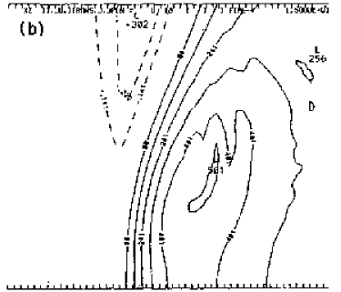
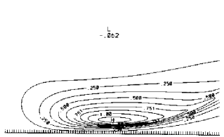
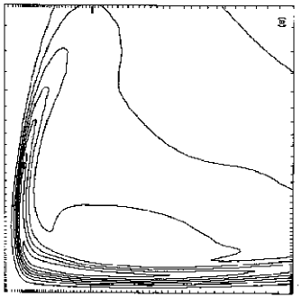
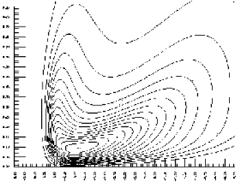
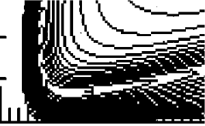
Based on the comparisons of resolutions in Kerr (1993) and the pseudospectral test just mentioned, the evidence is that Kerr (1993) is resolved at least until $t=16.5$. Fig. 2, take from Kerr (1993) at $t=15<16.5$, shows that the innermost vorticity contour is in the corner. In Fig. 14, taken from Fig. 15 of Hou & Li (2006), the innermost contour is flattened.

What the contours from Hou & Li (2006) most resemble are the later times from the unfiltered calculation from Kerr (1992) in Fig. 8 and $t>8.2$ from Pumir & Siggia (1990) shown in Fig. 11. This suggests that noise at the small scales that becomes amplified is the source of the differences. Since they do filter their initial condition, where does the necessary noise come from? The most likely source would be retaining wavenumbers beyond the 2/3rds rule cutoff.

The simplest test of this proposal would be to check for small negative regions of vorticity, locate them, and plot how they grow in time. Our plan is to run independent calculations to check this possibility.

Another sign of a difference for $t<17$ is obtained by comparing the behavior of enstrophy and its production plotted in Fig 15. Upon my suggestion, Hou & Li (2006) added the time dependence of enstrophy $\Omega$ and enstrophy production $\Omega_{pr}$ to the version they submitted. The units are not those used by Kerr (1993), so in Fig 15 the assumption is made that the Kerr (1993) and Hou & Li (2006) calculations are identical for $t<10$ and therefore by scaling their values at $t=10$, a comparison can be made. The discussion in Hou & Li (2006) suggests that the values of $\Omega_{pr}$ shown were calculated from $(d/dt)\Omega$ and not from $\int dV\omega_{i}e_{ij}\omega_{j}$ directly.

Both $\Omega$ and $\Omega_{pr}$ grow faster than in Kerr (1993) for $12<t<16$ and then more slowly. This is seen best in the third figure for $\Omega_{pr}$. This trend would be consistent with there being more enstrophy growth in the long tail initially, but less concentration in the corner to build upon at later times. In the table below the numbers used to make these plots are given. The enstrophy results from Kerr (1993) correct a misprint. The formula for enstrophy in Kerr (1993) should have been: $\Omega=-.0105\log(18.9-t)+.05$, giving $\Omega(t=0)=.019$.

$$\begin{array}[]{ccccc}&{\rm Chebyshev}&t_{c}=18.9&{\rm Hou\&Li}&t_{c}=18.7\\ {\rm time}&15.5&17.5&15&17.5\\ \Omega&.0375&.0507&6.9&9.8\\ t_{c}-t&3.4&1.4&3.7&1.2\\ \log(t_{c}-t)&1.22&.336\\ \Omega_{pr}&.00158&.00375&.6&1.95\end{array}$$

7 Moving forward

In March 2003, A. Bhattacharee, U. Frisch, R.M. Kerr, N. Zabusky and others met at the Institute for Advanced Studies in Princeton to consider what direction a new computational effort should follow. This meeting was instigated by the untimely death of our friend and collegue Rich Pelz.

The primary conclusion that was reached was that there was a serious problem where each numerical method seemed to give a different answer. It was concluded that this was primarily because each team was pushing their calculations a little too far. In the early 1990s there was really no choice. To get any trend one had to overextend the calculations. In the first decade of the 21st century there is the luxury of far greater computing power and significantly improved numerical methods. Therefore it was decided to propose an international collaborative effort based on:

• A factor of at least 4 increase in resolution in each direction

• Availability of modern adaptive mesh finite difference and spectral element codes capable of providing significant improvements in local resolution.

• Separate groups should conduct simultaneous simulations with the same initial conditions. The only results that should be reported are until a time when the two calculations differ only by an agreed upon amount.

Only in the UK was a proposal made. A separate proposal with no communication with the people above, and therefore not informed of the rules, was funded and went to T. Hou at Cal Tech, R. Caflisch at UCLA and M. Siegel at the New Jersey Institute of Technology. The UK proposal between Warwick and Imperial was never funded due to the poor rules for reviewing interdisciplinary proposals in the UK. Funding has finally been obtained from the Leverhulme Foundation, but only for one post-doc at Warwick.

The original intention was that the two first adaptive codes to be used would be the spectral element code of Barkley at Warwick and some variant of the finite-difference adaptive code of Grauer in Bochum or from within Bhattacharjeee’s group at New Hampshire. Later, the improved spectral element code of Sherwin from Imperial would be used.

Most likely at this time we will go directly to Sherwin’s spectral element code and work with Pumir on reviving his adaptive-mesh finite difference code.

However, the first priority now is to address the issues raised by Hou & Li (2006). Therefore, their calculations will be repeated and compared in detail with a straight pseudospectral calculation using a strict 2/3rds rule and stopped early enough so that there are no questions about small-scale resolution. This should be near $t=17$, although the comparison above suggests that a difference should show up as early as $t=15$.

References

- Ashurst & Meiron (1987) Ashurst, W., & Meiron, D. 1987 Numerical study of vortex reconnection. Phys. Rev. Lett. 58, 1632–1635.
- Beale et al. (1984) Beale, J. T., Kato, T., & Majda, A. 1984 Remarks on the breakdown of smooth solutions for the Euler equations. Commun. Math. Phys. 94, 61.
- Boratav et al. (1992) Boratav, ON, Pelz, RB, & Zabusky, NJ 1992 Reconnection in orthogonally interacting vortex tubes: Direct numerical simulations and quantification in orthogonally interacting vortices. Phys. Fluids A 4, 581–605.
- Brachet et al. (1983) Brachet, M.E., Meiron, D.I., Orszag, S. A.,Nickel, B. G., Morf, R.H., & Frisch, U. 1983 Small-scale structure of the Taylor-Green vortex. J. Fluid Mech. 130, 411-452.
- Caffarelle et al. (1982) Caffarelle, L., Kohn, R., & Nirenberg, L. 1982 . Commun. Pure Appl. Math. 35, 771.
- Constantin et al. (1996) Constantin, P., Fefferman, C., & Majda, A. 1996 Geometric constraints on potentially singular solutions for the 3D Euler equations. Comm. Partial. Diff. Equns. 21, 559-571.
- Grauer et al. (1998) Grauer, R., Marliani, C., & Germaschewski, K. 1998 Adaptive mesh refinement for singular solutions of the incompressible Euler equations.. Phys. Rev. Lett. 80, 4177–4180.
- Hou & Li (2006) Hou, T.Y., & Li, R. 2006 J. Nonlin. Sci.. Dynamic depletion of vortex stretching and non-blowup of the 3-D incompressible Euler equations (submitted).
- Kerr (1992) Kerr, R.M. 1992 Evidence for a singularity of the three-dimensional incompressible Euler equations.. In Topological aspects of the dynamics of fluids and plasmas (ed. G.M. Zaslavsky, M. Tabor & P. Comte), pp. 309–336. Proceedings of the NATO-ARW workshop at the Institute for Theoretical Physics, University of California at Santa Barbara. Kluwer Academic Publishers, Dordrecht, Netherlands..
- Kerr (1993) Kerr, R.M. 1993a Evidence for a singularity of the three-dimensional, incompressible Euler equations. Phys. Fluids A 5, 1725–1746.
- Kerr (2005) Kerr, R.M. 2005 Velocity and scaling of collapsing Euler vortices. Phys. Fluids 17, 075103.
- Kerr & Hussain (1989) Kerr, R.M., & Hussain, F. 1989 Simulation of vortex reconnection. Physica D 37, 474-484.
- Melander & Hussain (1989) Melander, M.V., & Hussain, F. 1989 Cross-linking of two antiparallel vortex tubes. Phys. Fluids A 1, 633-636.
- Pelz (2001) Pelz, R. 2001 Symmetry and the hydrodynamic blow-up problem. J. Fluid Mech. 444, 299-320.
- Ponce (1985) Ponce, G. 1985 Remark on a paper by J.T. Beale, T. Kato and A. Majda. Commun. Math. Phys. 98, 349.
- Pumir & Kerr (1987) Pumir, A., & Kerr, R. M. 1987 Numerical simulation of interacting vortex tubes. Phys. Rev. Lett. 58, 1636–1639.
- Pumir & Siggia (1987) Pumir, A., & Siggia, E. D. 1987 Vortex dynamics and the existence of solutions of the Navier-Stokes equations. Phys. Fluids 30, 1606-1626.
- Pumir & Siggia (1990) Pumir, A., & Siggia, E. D. 1990 Collapsing solutions to the 3-D Euler equations. Phys. Fluids A 2, 220–241.
- Shelley et al. (1993) Shelley, M.J., Meiron, D.I., & Orszag, S.A. 1993 . J. Fluid Mech. , 246-613.
- Sulem et al. (1985) Sulem, P.L., Frisch, U., Pouquet, A., & Meneguzzi, M. 1985 . J. Plasma Phys. 33, 191.
- Kerr (2006) Kerr, R.M. 2006 Computational Euler History. Identical text with cleaner figures are in: http://www.eng.warwick.ac.uk/staff/rmk/rmk_pubs/compEulerhist_arXiv.pdf