High-Frequency Acoustic Sediment Classification in Shallow Water

Abstract

A geoacoustic inversion technique for high-frequency (12 kHz) multibeam sonar data is presented as a means to classify the seafloor sediment in shallow water (40–300 m). The inversion makes use of backscattered data at a variety of grazing angles to estimate mean grain size. The need for sediment type and the large amounts of multibeam data being collected with the Naval Oceanographic Office’s Simrad EM 121A systems, have fostered the development of algorithms to process the EM 121A acoustic backscatter into maps of sediment type. The APL-UW (Applied Physics Laboratory at the University of Washington) backscattering model is used with simulated annealing to invert for six geoacoustic parameters. For the inversion, three of the parameters are constrained according to empirical correlations with mean grain size, which is introduced as an unconstrained parameter. The four unconstrained (free) parameters are mean grain size, sediment volume interaction, and two seafloor roughness parameters. Acoustic sediment classification is performed in the Onslow Bay region off the coast of North Carolina using data from the 12kHz Simrad EM 121A multibeam sonar system. Raw hydrophone data is beamformed into 122 beams with a 120-degree swath on the ocean floor, and backscattering strengths are calculated for each beam and for each ping. Ground truth consists of 68 grab samples in the immediate vicinity of the sonar survey, which have been analyzed for mean grain size. Mean grain size from the inversion shows 90% agreement with the ground truth and may be a useful tool for high-frequency acoustic sediment classification in shallow water.

I Introduction

The U. S. Navy has great interest in seafloor characterization due to its importance in shallow-water operations, such as landing operations, mine burial, and safety of navigation. Determining a suitable route for communications cables, requires detailed knowledge of the seafloor and is another application for characterization of the ocean bottom.

Obtaining and analyzing physical core samples or grab samples provides an accurate characterization of the seafloor, however, it is a time-consuming process and is not generally performed with sufficient coverage on an ocean survey. As an alternative, acoustic seafloor characterization allows adequate coverage in much less time and, since sonar data is often collected on surveys, no additional data collection is required. The acoustic data evaluated in this paper was collected in Onslow Bay with the 12 kHz Simrad EM 121A Multibeam Echo Sounder.

I-A Sediment Types

One of the most useful descriptors for bottom characterization is sediment type based on the mean grain diameter, which can range from clay ($\approx$ 0.0039 mm) to boulders ($\approx$ 256 mm) or greater. A phi value $\phi$ scale conveniently represents the mean grain size according to

$$\phi=-\log_{2}\frac{d}{d_{0}},$$ (1)

where $d$ is the mean grain diameter in mm and $d_{0}$ is the reference diameter 1 mm. Approximate $\phi$ values for selected sediments are given in Table I according to the Wentworth scale [2].

TABLE I: Sediment Types

Phi Value $\phi$	Mean Grain Diameter	Sediment Type
	(mm)
$\leq$ ($-1.0$)	$\geq 2.0$	gravel/rock
($-1.0$) – $4.0$	$0.06$ – $2.0$	sand
$4.0$ – $8.0$	$0.004$ – $0.06$	silt
$>8.0$	$<0.004$	clay

I-B Onslow Bay

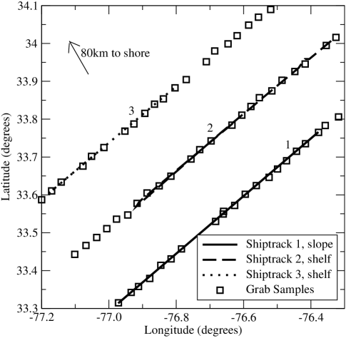
Onslow Bay off the coast of North Carolina is a challenging region for high-frequency acoustic sediment classification because the bottom is dynamic (sediment drift) [3], heterogeneous in areas [4, 5] with shells, etc., mixed with the sediment, and is often composed of a hard bottom [5, 6] covered with only a thin (few centimeters or less) layer of sediment. The sonar data set from this survey is raw hydrophone data along the three parallel shiptracks depicted in Fig. 1 that are more or less parallel to the coastline. Shiptrack 1 has 250 – 300 m water depth and is farthest from shore near the continental-shelf break. The seafloor slopes up to 0.5^∘ in a direction perpendicular to the ship’s heading. Shiptracks 2 and 3 are in shallower water (40 – 60 m) about 80km from shore, seafloor here on the shelf is relatively flat.

Figure 1: Shiptracks and collocated grab samples in the Onslow Bay area.

I-C Hydrophone Data Processing

Each port and starboard arrays are comprised of 64 hydrophones. Each array is steered between -60 and 60 degrees (negative being in the port direction) in one-degree increments. However, both port and starboard arrays are steered at 0 degrees so there are 122 steer directions (beams).

I-C1 Preprocessing

For each ping, header, raw data, and PAM (Power Amplifier Monitor) records are read from the tape or a file. A number of samples (usually 1028) from each ping are taken from the raw data record. Where applicable the beginning sample is selected according to the value of the Time-Varying Gain TVG and a hard-coded threshold. The effects of Programmable Gain PG, Fixed Gain FG, and Time-Varying Gain TVG are removed from the data. These computations are made in linear space based on values obtained from the header record. The data, now in units of digital number DN, are converted to sound pressure level SPL. Values for this conversion are taken from the header record.

At this point the data are still at baseband. To beamform, the data are shifted to the original center frequency (12 kHz). To avoid aliasing the basebanded data must be resampled at a higher rate than the original sampling rate of 2.5 kHz. The resample factor used is 16, so the resampling rate is 40 kHz. The interpolation is done via a Fast Fourier Transform (FFT). The slow data are transformed to the frequency domain with a large FFT, shifted, then transformed back to the time domain.

After the shift to 12 kHz, the average roll, pitch, heave and yaw for the given ping are computed. These values are then used to adjust the absolute locations (in software) of the receiver staves in the array and will enable the beams to be steered to consistent beam angles relative to the seafloor.

Following the motion correction the data are beamformed by phase adjusting the frequency domain data according to the receiver locations and desired steering angles. Taking the inverse FFT of these data yields a sound pressure $P$ time series for each steering angle. The travel time of the bottom return is identified for each angle and an acoustic ray is traced out (here a constant sound speed profile is used because of a negligible sound speed gradient) to the corresponding bottom returns in order to obtain grazing angle.

The sound pressure for the $j$th time sample of the $i$th beam is denoted $P_{ij}$. The data are converted to dB re $\mu$Pa and, based on the known geometry, the sonar equation is solved for bottom backscatter.

I-C2 Backscattering Strength

Backscattering strength $BS$ is defined as

$$BS=10\log_{10}\frac{I_{b}}{I_{inc}},$$ (2)

where $I_{b}$ is the backscattered sound intensity from an area of 1 m² and $I_{inc}$ is the incident intensity at 1 m from the source [7]. The backscattering strength can be determined from the data by using the sonar equation

$$BS=RL-SL+2TL-IA,$$ (3)

where $RL$ is the reverberation level (from the beamformed time series), $SL$ is the source level, $TL$ is the transmission loss in dB, and $IA$ is the insonified area in dB re m². The insonified area is the area contributing to the received intensity and is computed using the 3 dB beam footprint,

$$IA=10\log_{10}\biggl{\{}2R^{2}\sin\frac{\theta_{t}}{2}\biggl{[}\cot\biggl{(}\theta+\frac{\theta_{r}}{2}\biggr{)}-\cot\biggl{(}\theta-\frac{\theta_{r}}{2}\biggr{)}\biggr{]}\sin\theta\biggr{\}},$$ (4)

or using the pulse length,

$$IA=10\log_{10}\biggl{(}\frac{c\tau R\sin\frac{\theta_{t}}{2}}{\cos\theta}\biggr{)},$$ (5)

whichever is smaller, where $R$ is the slant range to the bottom, $\theta_{t}$ is the transmit beam width, $\theta_{r}$ is the receive beam width, $c$ is the water sound speed in m/s, and $\tau$ is the pulse duration in s. The insonified area for several pressure time samples $P_{ij}$ normally fall within the beam footprint, and the reverberation level for the $i$th beam $RL_{i}$ is averaged over these time samples,

$$RL_{i}=10\log_{10}\biggl{(}\frac{\sum_{j_{0}}^{j_{1}}P_{ij}^{2}}{j_{1}-j_{0}+1}\biggr{)},$$ (6)

where $j_{0}$ and $j_{1}$ are the first and last time samples whose insonified areas lie within the $i$th beam’s footprint.

TABLE II: Model Input Parameters

Parameter	Symbol	Description
Density Ratio	$\rho$	$\frac{\hbox{density in sediment}}{\hbox{density in water}}$
Sound Speed Ratio	$\nu$	$\frac{\hbox{sound speed in sediment}}{c}$
Loss Parameter	$\delta$	$\frac{\hbox{imaginary wavenumber in sediment}}{\hbox{real wavenumber}}$
Spectral Strength	$\beta$	Bottom height spectrum strength
Spectral Exponent	$\gamma$	Bottom height spectrum exponent
Volume Parameter	$\sigma$	$\frac{\sigma_{v}}{\hbox{sediment attenuation coefficient}}$

II Backscatter Model

The APL-UW backscatter model presented by Mourad and Jackson [8, 9] treats the seafloor as a statistically homogeneous fluid and predicts backscattering strength $BS$ as a function of grazing angle $\theta$. The roughness of the bottom is described in this model by the bottom height spectrum.

$$W=\beta\biggl{(}\frac{2\pi fh}{c}\biggr{)}^{-\gamma},$$ (7)

where $h$ is the reference height 1cm. The Mourad-Jackson model is valid for all frequencies between 10 and 100 kHz and is used here to represent the acoustic backscatter from the seafloor.

Table II lists the six model input parameters, which, along with the sonar frequency $f$ and sound speed $c$ in water at the seafloor, determine both the roughness backscattering cross section $\sigma_{r}(\theta)$ and volume backscattering cross section $\sigma_{v}(\theta)$. The six input parameters are dimensionless except for $\beta$ which has units of cm⁴. Combining these backscatter contributions from roughness (acoustic reflections from a randomly rough surface) and volume interaction (scattering of penetrating sound from sediment inhomogeneities) results in

$$BS(\theta)=10\log_{10}(\sigma_{r}+\sigma_{v}).$$ (8)

III Data Inversion

The inversion problem is finding the set of input parameters that best fits the given data set. That is, which set of parameters minimizes the difference between the $BS$ vs. $\theta$ curve and the measured backscatter data. The sum of the squares of the data deviations from the model prediction is used as the measure for goodness of fit.

III-A Parameter Constraints

If the six input parameters are unconstrained, the parameter space to be searched is six-dimensional. However, since correlations exist among some of the parameters, many solution parameter sets represent solutions that are physically unlikely. Hamilton and Bachmann [10, 11] describe a relationship between the parameters $\rho$ and $\nu$ and relate both to the mean grain size ($\phi$) of the seafloor sediments. Mourad and Jackson [8] parameterize $\rho$, $\nu$, and $\delta$ according to $\phi$ values emphasizing the top few tens of centimeters of sediment, and the parameterization has been generalized to include coarse sand [9]. (Some correlation exists between $\delta$ and $\phi$, and the effect of physically meaningful values of $\delta$ on the $BS$ vs. $\theta$ curve is negligible.) Gott [12] has used the idea of constraining some of the model parameters with some success. In addition the parameters used should be restricted to values that are physically likely. The parameter ranges used here are presented in Table III.

TABLE III: Parameters Ranges

Parameter	Range
$\phi$	($-1.0$) – $9.0$
$\beta$	within factor of 2 of APL-UW
	parameterization [9]
$\gamma$	$2.4$ – $3.9$
$\sigma$	$0.00$ – $0.02$

The parameter space to be searched is now 4-dimensional ($\phi$, $\beta$, $\gamma$, $\alpha$), and, since the backscatter model is highly nonlinear, one must be careful not to simply find one of the many local solutions. Two of the most common global search methods are simulated annealing and genetic algorithms. Both are suitable for most nonlinear problems. Simulated annealing (SA) is the best-fit search routine used here (e.g. see [13]).

III-B Simulated Annealing

With the SA approach one searches the parameter space by continuously stepping to a new point in parameter space and computing the sum of the squares $E$ for the data point residuals. $E$ is also known as the cost function. If the cost decreases from the previous location, the step is accepted. If, however, the cost increases, the step is only occasionally accepted. The probability $p$ that a higher-cost step is accepted depends both on the amount of increased cost $\Delta E$ and on a variable referred to as temperature $t$ according to the Boltzmann distribution,

$$p=e^{-\Delta E/t}.$$ (9)

This process is known as the Metropolis algorithm [14]. Local minima are escaped because of the steps of increased cost. The temperature variable is gradually decreased until the probability of a higher-cost step is zero. The stepsize is also reduced slowly as the algorithm settles into the global minimum.

IV Results

IV-A Slope Region

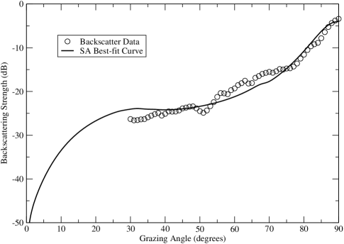
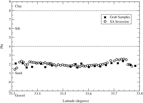
The data for shiptrack 1 (farthest from shore) was grouped into bins of 200 pings covering an area of seafloor approximately 3 km$\times$1 km. The backscattering strengths in each bin were averaged according to grazing angle, and a best-fit parameter set was found via simulated annealing for the averaged data. To illustrate Fig. 2 shows backscatter data for the first 200 pings for shiptrack 1 along with the SA best-fit model curve. A comparison of inversion phi values with the analyzed grab samples is shown in Fig. 3. All 58 inversions for the 200-ping bins result in phi values indicating medium or fine grades of sand. The inversion phi values are in most cases only slightly greater than medium sand measured at the nearest grab sample location.

Figure 2: Backscatter data from the first 200 pings from shiptrack 1 and the best-fit model curve. The inversion indicates $\phi=1.41$, while the nearest grab sample shows $\phi=2.08$.

Figure 3: Comparison of phi values from inversion with the measured grab samples in the slope region.

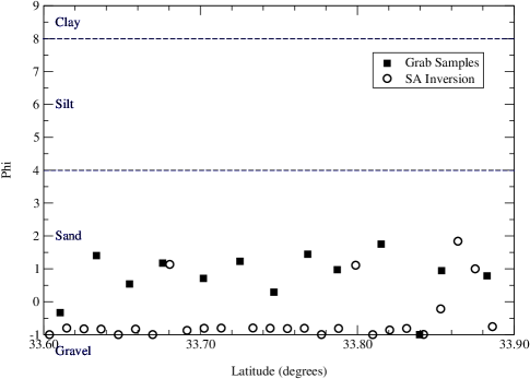
IV-B Shelf Region

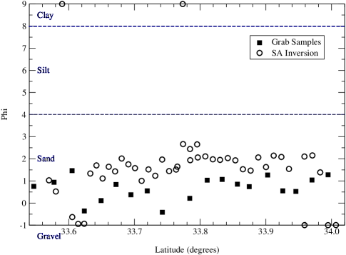
Because of a higher ping rate, the backscatter data from shiptracks 2 and 3 are binned in groups of 500 pings each. Figures 4 and 5 (closest to shore) compare the phi values from the SA inversion to the grab samples in the shallower water ($\approx$ 40–60 m) with 61 of the 71 inversion phi values matching the nearest grab sample sediment type. Forty-three grab samples in the shelf region show a medium or coarse sand bottom with one sample indicating gravel. The inversion yields 60 sand, 9 gravel, and 2 clay values. This region exhibits greater variation in phi values than the slope region.

Figure 4: Comparison of phi value from inversion with grab sample analysis in the shelf region along shiptrack 2.

Figure 5: Comparison of phi value from inversion with grab sample analysis in the shelf region along shiptrack 3.

TABLE IV: Average Phi Values

Region	Grab Samples	Inversion	Sediment Type	% Agreement
Slope	$1.92\pm 0.36$	$2.02\pm 0.24$	Medium–fine sand	$100\%$
Shelf	$0.82\pm 0.71$	$0.92\pm 2.04$	Medium–coarse sand	$86\%$

V Conclusions

The inversion results are in good agreement with the ground truth (both in sediment type, i.e, sand, and in grade of sand) for the slope region where the sediment layer is known to be relatively deep and homogeneous (near the continental shelf break). The seafloor in the shelf area, on the other hand, is known to have little or no sediment layer and shells, rocks, etc., at the bottom. The inversion from the shelf region also agrees in sediment type with most grab samples, however, there is often a discrepancy in grade of sand. Moreover, in a few cases the phi value from the inversion is the lower limit (-1, i.e., gravel/coarse sand). Because the sonar frequency is 12 kHz, the sound will penetrate any sediment layer less than about 13 cm (wavelength) deep and interact with the hard subbottom. The backscattering strength predicted by the APL-UW model in this case will be invalid.

Of the 129 inversions for the three shiptracks, 119 of them (92%) agree with the nearest grab sample in sediment type. Average values and standard deviations are listed in Table IV along with the percent agreement of the inversion phi values with the nearest grab sample.

We believe the inversion method described here is promising for determining sediment type in areas of relatively homogeneous sediment and at least a few tens of centimeters deep. This process currently also provides an approximation for thin sediment layers or sediment with heterogeneous mixtures.

References

- [1]
- [2] C. K. Wentworth, “A scale of grade and class for clastic sediments,” J. Geology, vol. 30, p. 377, 1922.
- [3] S. R. Riggs, W. G. Ambrose, J. W. Cook, S. W. Snyder, and S. W. Snyder, “Sediment production on sediment-starved continental margins: The interrelationship between hard-bottoms, sedimentological and benthic community processes, and storm dynamics,” J. Sedimentary Research vol. 68, p. 155 (1998).
- [4] W. J. Cleary and O. H. Pilkey, J. Southeastern Geology vol. 9, p. 1, (1968).
- [5] J. T. DeAlteris, “Geology of Offshore Onslow Bay, North Carolina,” unpublished.
- [6] S. R. Riggs, S. W. Snyder, A. C. Hine, and D. L. Mearns, “Hardbottom morphology and relationship to the geologic framework: Mid-atlantic continental shelf,” J. Sedimentary Research vol. 66, p. 830 (1996).
- [7] R. J. Urick, Principles of Underwater Sound. Peninsula: Los Altos, 1983, pp. 238–239.
- [8] P. D. Mourad and D. R. Jackson, “High frequency sonar equation models for bottom backscatter and forward loss,” in Proceedings of OCEANS ’89 (IEEE, New York, 1989), pp. 1168–1175.
- [9] “APL-UW High-Frequency Ocean Environmental Acoustic Models Handbook,” Applied Physics Laboratory, University of Washington, Seattle, WA, Tech. Rep. TR-9407, Oct. 1994.
- [10] E. L. Hamilton, “Compressional-wave attenuation in marine sediments,” Geophysics vol. 37, p. 620 (1972).
- [11] E. L. Hamilton and R. T. Bachmann, “Sound velocity and related properties of marine sediments,” J. Acoust. Soc. Am. vol. 72, p. 1891 (1982).
- [12] R. M. Gott, Remote Seafloor Classification Using Multibeam Sonar, Ph.D. thesis, Tulane University (1995).
- [13] W. H. Press, S. A. Teukolsky, W. T. Vetterling, and B. P. Flannery, Numerical Recipes in Fortran 77: The Art of Scientific Computing, 2nd ed. Cambridge: Cambridge, 1992.
- [14] N. Metropolis, A. W. Rosenbluth, M. N. Rosenbluth, A. H. Teller, and E. Teller, J. Chem. Phys. vol. 21, p. 1087 (1953).