Electrostatic internal energy using the method of images

Abstract

For several configurations of charges in the presence of conductors, the method of images permits us to obtain some observables associated with such a configuration by replacing the conductors with some image charges. However, simple inspection shows that the potential energy associated with both systems does not coincide. Nevertheless, it can be shown that for a system of a grounded or neutral conductor and a distribution of charges outside, the external potential energy associated with the real charge distribution embedded in the field generated by the set of image charges is twice the value of the internal potential energy associated with the original system. This assertion is valid for any size and shape of the conductor, and regardless of the configuration of images required. In addition, even in the case in which the conductor is not grounded nor neutral, it is still possible to calculate the internal potential energy of the original configuration through the method of images. These results show that the method of images could also be useful for calculations of the internal potential energy of the original system.

Keywords: method of images, potential energy, electrostatics, boundary conditions.

PACS: 41.20.Cv, 01.40.Fk, 01.40.gb

The method of images is a useful tool to calculate electrostatic fields, Green functions and forces that conductors of certain shapes exert over some charges [1]-[3]. However, the internal energy of the configuration is seldom treated by this method [4], and applications are restricted to very special cases [3]. Let us call system A (the real system) the one consisting of a conductor and certain distribution of charges outside it, and system B (the virtual system) the one consisting of the distribution of charges plus the set of image charges, see Fig. 1. The reason that prevents us from calculating the energy of system A based on system B, is that the integral $\int\mathbf{E}^{2}dV$ is not the same for both configurations, because in the region inside the conductor the electric field is different in each system. For an arbitrary size and shape of the conductor there is no evident symmetry to connect the energies of both configurations. Remarkably, despite the lack of symmetry, it can be demonstrated that for system A with the conductor grounded or neutral, the external potential energy associated with the real distribution of charges in the presence of the set of images is twice the value of the internal potential energy associated with system A. This fact is true for an arbitrary size and shape of the conductor, and whatever the configuration of images is. Therefore, the method of images could also be utilized for calculations of the internal potential energy of the original system. Finally, the result could be extended for the case in which the conductor is not neccesarily grounded nor neutral.

Figure 1: System A is defined as the set composed of the conductor and the distribution of charges $\left\{q_{j}\right\}$ outside the conductor (left). System B consists of the distribution of charges $\left\{q_{j}\right\}$ plus the set of image charges $\left\{\bar{q}_{k}\right\}$, (right)

1 General approach

We want to find the internal potential energy associated with a system consisting of a point charge $q$ in the presence of a conductor (system A); we shall start from the expression

$$U_{int}^{\left(A\right)}=\frac{1}{2}\int\rho\left(\mathbf{r}\right)\ \phi\left(\mathbf{r}\right)\ dV,$$ (1)

where $\rho\left(\mathbf{r}\right),\ \phi\left(\mathbf{r}\right)$ denote the charge density and potential, respectively. It is well known that Ec. (1) leads to divergences when point particles are present because of the inclusion of self energy terms [3]. Of course, the self energy term can be removed to get only finite results. Extracting the self energy and taking into account that the integral only contributes in regions where charge is present, we get

$$U_{int}^{\left(A\right)}=\frac{1}{2}q_{c}\phi_{s}+\frac{1}{2}q\phi_{A}\left(\mathbf{r}_{0}\right),$$ (2)

where $\phi_{s}$ is the potential on the surface of the conductor, $\mathbf{r}_{0}$ describes the location of the point charge, $q_{c}$ is the net charge of the conductor, and $\phi_{A}\left(\mathbf{r}_{0}\right)$ is the electric potential at $\mathbf{r}_{0}$ due to all sources (excluding $q$ itself i.e. removing the divergence). From the method of images [1]-[3], the electric potential outside the conductor is equivalent to the electric potential generated by system B (the charge $q$ plus the set of images). In particular, the electric potential generated by the set of image charges at the point $\mathbf{r}_{0}$ is given by

$$\phi_{B}\left(\mathbf{r}_{0}\right)=\sum_{k=1}^{N}\frac{K_{c}\bar{q}_{k}}{\left|\mathbf{\bar{r}}_{k}-\mathbf{r}_{0}\right|}=\phi_{A}\left(\mathbf{r}_{0}\right)\ ,$$ (3)

where $\left(\bar{q}_{k},\mathbf{\bar{r}}_{k}\right)$ denotes the set of image charges and their positions, and $K_{c}\equiv\left(4\pi\varepsilon_{0}\right)^{-1}$ in SI units. Replacing (3) into (2) we find

$$U_{int}^{\left(A\right)}=\frac{1}{2}q_{c}\phi_{s}+\frac{1}{2}\left[\sum_{k=1}^{N}\frac{K_{c}\bar{q}_{k}q}{\left|\mathbf{\bar{r}}_{k}-\mathbf{r}_{0}\right|}\right]\ .$$ (4)

From Gauss’s law, it can be seen that the net charge $q_{c}$ on the surface of the conductor is the algebraic sum of the image charges. Similarly, the potential on the surface of the conductor is the potential generated by system B in any point of such a surface; hence we get

$$q_{c}=\sum_{k=1}^{N}\bar{q}_{k}\ \ ;\ \ \phi_{s}=\frac{K_{c}q}{\left|\mathbf{r}_{0}-\mathbf{r}_{s}\right|}+\sum_{k=1}^{N}\frac{K_{c}\bar{q}_{k}}{\left|\mathbf{\bar{r}}_{k}-\mathbf{r}_{s}\right|}\ ,$$ (5)

where $\mathbf{r}_{s}$ is the position of any point on the surface of the conductor. Replacing (5) into (4), we get the internal energy of system A in terms of the components of system B

$$U_{int}^{\left(A\right)} = \frac{1}{2}\left(\sum_{k=1}^{N}\bar{q}_{k}\right)\left(\frac{K_{c}q}{\left|\mathbf{r}_{0}-\mathbf{r}_{s}\right|}+\sum_{m=1}^{N}\frac{K_{c}\bar{q}_{m}}{\left|\mathbf{\bar{r}}_{m}-\mathbf{r}_{s}\right|}\right)$$ (6)

$$+\frac{1}{2}\left[\sum_{k=1}^{N}\frac{K_{c}\bar{q}_{k}q}{\left|\mathbf{\bar{r}}_{k}-\mathbf{r}_{0}\right|}\right].$$

The term in square brackets in Eq. (6) is the potential energy associated with the point charge $q$ in the presence of the set of images, which we shall denote as $U_{q}^{\left(B\right)}$ getting

$$U_{int}^{\left(A\right)}=\frac{1}{2}q_{c}\phi_{s}+\frac{1}{2}U_{q}^{\left(B\right)}.$$ (7)

Equation (7) is valid for an arbitrary form of the conductor, and allows us to find the internal potential energy of the real system, based on the potential energy associated with the point charge $q$ in the presence of the image charges. Result (7) can be further generalized by using the principle of superposition. So if instead of a point charge we have a distribution of $M$ charges denoted by $\left\{q_{j}\right\}$, Eq. (7)  becomes

$$U_{int}^{\left(A\right)} = \frac{1}{2}q_{c}\phi_{s}+\frac{1}{2}U_{ext}^{\left(B\right)}\ ,$$

$$q_{c} = \sum_{k=1}^{N}\bar{q}_{k}\ \ ;\ \ \phi_{s}=\sum_{j=1}^{M}\frac{K_{c}q_{j}}{\left|\mathbf{r}_{j}-\mathbf{r}_{s}\right|}+\sum_{m=1}^{N}\frac{K_{c}\bar{q}_{m}}{\left|\mathbf{\bar{r}}_{m}-\mathbf{r}_{s}\right|}$$

$$U_{ext}^{\left(B\right)} \equiv \sum_{j=1}^{M}q_{j}\sum_{k=1}^{N}\frac{K_{c}\bar{q}_{k}}{\left|\mathbf{\bar{r}}_{k}-\mathbf{r}_{j}\right|}=\sum_{j=1}^{M}q_{j}\bar{\phi}\left(\mathbf{r}_{j}\right)\ ,$$ (8)

where $\bar{\phi}\left(\mathbf{r}_{j}\right)$ is the potential generated by the set of images in the location $\mathbf{r}_{j}$ of the charge $q_{j}$. Thus, $U_{ext}^{\left(B\right)}$ represents the external potential energy associated with the distribution of real charges when they are immersed in the field generated by the images. Of course, the distribution (and perhaps the images) could also be continuous; in that case the sums become integrals. In particular, if the conductor is grounded or neutral we find that

$$U_{int}^{\left(A\right)}=\frac{1}{2}U_{ext}^{\left(B\right)}\ .$$ (9)

At this point it would be convenient to discuss briefly about the difference between external and internal potential energies [5]. First, we should precise the system of particles for which we define the concepts of external and internal. Once the system is defined, the internal potential energy is that associated with the internal forces and corresponds to the work necessary to ensemble the system starting from the particles far away from each other. On the other hand, the external potential energy is that associated with the external forces, and corresponds to the work necessary to bring the system as a whole from infinity to their final positions, immersed in the field of forces generated by all sources outside the system. In our case, $U_{ext}^{\left(B\right)}$ represents the external potential energy associated with the system of real charges in which the external forces are provided by the system of images. Therefore, $U_{ext}^{\left(B\right)}$ is the work necessary to bring the distribution $\left\{q_{j}\right\}$ as a whole, from infinity to their final positions in the presence of the image charges. On the other hand, $U_{int}^{\left(A\right)\text{ }}$ represents the work necessary to ensemble the system consisting of the conductor and the real charges which is the observable we are interested in. Note that internal and external potential energies are conceptually and operationally different.

2 Simple applications

We shall work on two types of scenarios (a) The conductor is isolated (so the net charge $q_{c}$ is fixed), and (b) The potential on the surface of the conductor is fixed (e.g. grounded or connected to a battery).

Example 1: The most typical problem treated by the method of images is the one of a point charge and an infinite grounded conducting plane. For many purposes, such a system is equivalent to replacing the conductor by the appropiate image charge, forming a physical dipole. Ref. [3], shows that the energy stored in system A, is only half of the energy stored in system B. It can be seen from either of the following arguments, (a) The space can be divided into two halves separated by the conductor. For system B the integral $\int\mathbf{E}^{2}dV$ gives identical contributions in both halves, while in system A only one of those halves contributes to the energy. (b) Calculating the work necessary to bring $q$ from infinity. In system A we only work on $q$ since the redistribution of charges in the conductor costs nothing because those charges are moving on an equipotential. By contrast, if we assemble system B by bringing both charges simultaneously, we could work on both of them symmetrically resulting in a work twice as great. This solution agrees with (9), and can be guessed by arguments of symmetry. However, Eq. (9) holds far beyond of this example.

Example 2: A point charge $q\$at $\mathbf{r}_{0}\$in the presence of an isolated, charged conductor with net charge $q_{c}$. We are interested in calculating the external work to bring $q$ from infinity to $\mathbf{r}_{0}$. The net charge is invariant during the process and the internal energy of the system at the beginning and at the end of the process are obtained by applying (4)

$$U_{int}^{\left(A,i\right)}=\frac{1}{2}q_{c}\phi_{s}^{i}\ ;\ U_{int}^{\left(A,f\right)}=\frac{1}{2}q_{c}\phi_{s}^{f}+\frac{1}{2}\left[\sum\limits_{k}\frac{K_{c}\bar{q}_{k}^{\left(f\right)}}{\left|\mathbf{r}_{0}-\mathbf{\bar{r}}_{k}^{\left(f\right)}\right|}q\right]\ ,$$

where $\phi_{s}^{i},\phi_{s}^{f}$ are the potentials on the surface of the conductor at the beginning and at the end of the process respectively, the set of images $\left\{\bar{q}_{k}^{\left(f\right)},\mathbf{\bar{r}}_{k}^{\left(f\right)}\right\}$ are those that fit the potential of the conductor at the end of the process (with $q$ lying at $\mathbf{r}_{0}$). We have assumed that the set of images is localized all over the process to ensure that the potential energy associated with the point charge is zero when it is located at infinity. The external work to bring $q$ from infinity to $\mathbf{r}_{0}$, is the change of internal energy

$$W_{ext}=\Delta U_{int}^{\left(A\right)}=\frac{1}{2}q_{c}(\phi_{s}^{f}-\phi_{s}^{i})+\frac{1}{2}\left[\sum\limits_{k}\frac{K_{c}\bar{q}_{k}^{\left(f\right)}}{\left|\mathbf{r}_{0}-\mathbf{\bar{r}}_{k}^{\left(f\right)}\right|}q\right]\ ,$$ (10)

the values of $\phi_{s}^{i}$ and $\phi_{s}^{f}$ can be obtained from Eq. (5) by utilizing the configuration of images at the beginning and at the end of the process respectively. It is clear that the values of $\phi_{s}^{f},\ \phi_{s}^{i}$ depend on the geometry of the conductor. Notice however that if the net charge is null, $W_{ext}$ becomes independent of those potentials and the result has the same form as that of the grounded conductor (see Eqs. 8, 9) regardless of the geometry of the conductor.

Example 3: Point charge $q$ at $\mathbf{r}_{0}$ with a conductor connected to a battery that keeps it at a fixed potential $V$. In the process of bringing $q\$from infinity to $\mathbf{r}_{0}$, the battery must supply a charge $\Delta Q$ to the conductor to maintain a constant voltage, so that applying (4) at the beginning and at the end and making the difference, we obtain the change in the internal energy

$$\Delta U_{int}^{\left(A\right)}=\frac{V}{2}\Delta Q+\frac{1}{2}\left[\sum\limits_{k}\frac{K_{c}\bar{q}_{k}^{\left(f\right)}}{\left|\mathbf{r}_{0}-\mathbf{\bar{r}}_{k}^{\left(f\right)}\right|}q\right]\ .$$

Again, we have assumed that the set of images is localized all over the process. Let us denote $q_{c}^{\left(i\right)},q_{c}^{\left(f\right)}$ as the total charges on the surface of the conductor at the beginning and at the end of the process respectively. Using Eq. (5), the change in internal energy becomes

$$\Delta U_{int}^{\left(A\right)} = \frac{V}{2}\left[\left(\sum_{k}\bar{q}_{k}^{\left(f\right)}\right)-\left(\sum_{m}\bar{q}_{m}^{\left(i\right)}\right)\right]$$ (11)

$$+\frac{1}{2}\left[\sum\limits_{k}\frac{K_{c}\bar{q}_{k}^{\left(f\right)}}{\left|\mathbf{r}_{0}-\mathbf{\bar{r}}_{k}^{\left(f\right)}\right|}q\right]\ .$$

This change of internal energy is equal to the net external work on the system, which can be separated in the work done by the battery to supply charge to the conductor plus the work due to the external force acting on $q$

$$\Delta U_{int}^{\left(A\right)}=W_{ext}=W_{batt}+W_{F_{ext}}\ .$$

Further, the work done by the battery is

$$W_{batt}=V\ \Delta Q=V\left[\left(\sum_{k}\bar{q}_{k}^{\left(f\right)}\right)-\left(\sum_{m}\bar{q}_{m}^{\left(i\right)}\right)\right]\ ,$$ (12)

so that $W_{F_{ext}}$ reads

$$W_{F_{ext}} = \frac{V}{2}\left[\left(\sum_{m}\bar{q}_{m}^{\left(i\right)}\right)-\left(\sum_{k}\bar{q}_{k}^{\left(f\right)}\right)\right]$$ (13)

$$+\frac{1}{2}\left[\sum\limits_{k}\frac{K_{c}\bar{q}_{k}^{\left(f\right)}}{\left|\mathbf{r}_{0}-\mathbf{\bar{r}}_{k}^{\left(f\right)}\right|}q\right]\ ,$$

the grounded conductor is a special case with $V=0$.

Examples 2, 3 are valid for any size and shape of the conductor. Let us apply these results for a spherical conductor of radius $R$, with the origin at the center of the sphere.

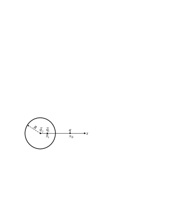
Figure 2: A point charge $q\$in the presence of a conducting sphere of radius $R$. The charges $\bar{q}_{1},\bar{q}_{2}$ are the set of images, and they acquire different values and positions according to the case studied. However $\bar{q}_{2}$ is always at the origin and the set $\bar{q}_{1},\bar{q}_{2},q$ lies on the $X-$axis.

Example 4: The sphere is connected to a battery that keeps its potential $V\$constant. The structure of the set of images is well known from the literature, (see for instance sections 2.2, 2.4 of [2]). In the notation of Fig. 2, for the charge $q$ at certain position $x_{0}$, the structure of the images is given by

$$\bar{q}_{1}=-\frac{qR}{x_{0}}\ ;\ \bar{x}_{1}=\frac{R^{2}}{x_{0}}\ ;\ \bar{q}_{2}=\frac{VR}{K_{c}}\ ;\ \bar{x}_{2}=0\ ,$$ (14)

the images at the beginning are obtained by taking $x_{0}\rightarrow\infty$, and at the end we just assume that the position is $x_{0}$; using (5) we find

$$q_{c}^{\left(i\right)}=\bar{q}_{1}^{\left(i\right)}+\bar{q}_{2}^{\left(i\right)}=\frac{VR}{K_{c}}\ ;\ q_{c}^{\left(f\right)}=\bar{q}_{1}^{\left(f\right)}+\bar{q}_{2}^{\left(f\right)}=-\frac{qR}{x_{0}}+\frac{VR}{K_{c}}$$ (15)

replacing (14, 15) into (12, 13) we find

$$W_{batt} = -\frac{qRV}{x_{0}}$$

$$\ W_{F_{ext}} = \frac{qRV}{x_{0}}-\frac{1}{2}\frac{K_{c}q^{2}R}{\left(x_{0}^{2}-R^{2}\right)}$$ (16)

$$= \frac{K_{c}\bar{q}_{2}q}{x_{0}}+\frac{1}{2}\frac{K_{c}q\bar{q}_{1}^{\left(f\right)}}{\left(x_{0}-\bar{x}_{1}^{\left(f\right)}\right)}\ .$$

the grounded sphere is obtained by setting $V=0$ (or $\bar{q}_{2}=0$). By examining the last line of Eq. (16) we see that the first term of $W_{F_{ext}}$ is equivalent to the work to bring the charge $q$ in the presence of the image $\bar{q}_{2}$ (which is invariant during the process). It is worth emphasizing that in this term the factor $1/2$ is not present because the charge $\bar{q}_{2}$ is stationary and constant in magnitude in the process of bringing $q$, so that the external force necessary to bring the charge is always of the form $K_{c}\bar{q}_{2}q/r^{2}$ in the direction of motion. By contrast, in the second term the factor $1/2$ is present and such a term is equivalent to half of the work required to carry the $q\$charge in the presence of the image $\bar{q}_{1}\$if such an image always remained in its final position, and with its final magnitude. This factor arises from the fact that during the process of bringing $q$, the image charge $\bar{q}_{1}$ must change its position and magnitude, in order to retain its role as image charge.

Example 5: The sphere is isolated with net charge $q_{c}$. Again, the structure of images required appears in the literature (see for instance sections 2.2, 2.3 of [2]), and in the notation of Fig. 2 they read

$$\bar{q}_{1}=-\frac{qR}{x_{0}}\ ;\ \bar{x}_{1}=\frac{R^{2}}{x_{0}}\ ;\ \bar{q}_{2}=q_{c}-\bar{q}_{1}=q_{c}+\frac{qR}{x_{0}}\ ;\ \bar{x}_{2}=0\ ,$$ (17)

the potential on the surface of the conductor when the charge lies in its final position, owes to the charge $\bar{q}_{2}$ only, since the potential generated by $\bar{q}_{1}$ and $q$ cancel each other by construction. On the other hand, the potential on the surface of the conductor when $q$ lies at infinity, is clearly of the form $K_{c}q_{c}/R$, and using (17) the potentials on the surface of the conductor at the beginning and at the end of the process read

$$\phi_{s}^{f}=\frac{K_{c}\bar{q}_{2}}{R}=\frac{K_{c}\left(q_{c}+\frac{qR}{x_{0}}\right)}{R}\ \ ;\ \ \phi_{s}^{i}\ =\frac{K_{c}q_{c}}{R}\ ,$$ (18)

replacing expressions (17, 18) into (10) we get

$$W_{ext}=K_{c}q\left\{\frac{q_{c}}{x_{0}}+\frac{qR}{2}\left[\frac{1}{x_{0}^{2}}-\frac{1}{\left(x_{0}^{2}-R^{2}\right)}\right]\right\}\ .$$

In this case, there is no work on the conductor similar to the case of a grounded sphere ($V=0$ in Eq. 16). In particular, in the scenario with a neutral conductor i.e. $q_{c}=0$, the work necessary to bring the charge is larger than in the case of a grounded sphere because a second image charge located at the centre and of the same sign of $q\$must be added, hence it leads to a repulsion that requires the external work to be increased.

Figure 3: An infinite wire with constant linear charge density $\lambda$, in front of a grounded conducting plane, and its corresponding image.

Example 6: Let us consider an infinite wire with uniform linear density $\lambda$, lying at a distance $a$ on the right-side of an infinite grounded conducting plane, see Fig. 3. In this case the image consists of another infinite wire of linear density $-\lambda$ on the left-side of the plane. In this example the real and image distributions are continuous. The electric potentials in a point $\mathbf{r=}x\mathbf{\hat{\imath}}+y\mathbf{\hat{\jmath}+}z\mathbf{\hat{k}}$ ($x>0$) due to the wire and its image are given by

$$\Phi(\mathbf{r}) = 2K_{c}\lambda\ln\sqrt{(x-a)^{2}+y^{2}}+C_{1},$$

$$\bar{\Phi}(\mathbf{r}) = -2K_{c}\lambda\ln\sqrt{(x+a)^{2}+y^{2}}+C_{2}.$$ (19)

To ensure that the potential over the plane is null ($YZ$ plane) we should choose the arbitrary constants as $C_{1}=-C_{2}=C$ so that the total potential on the right-side of the plane becomes

$$\Phi_{T}(\mathbf{r})=2K_{c}\lambda\ln\sqrt{\frac{(x-a)^{2}+y^{2}}{(x+a)^{2}+y^{2}}},$$

which satisfies the condition $\Phi_{T}(0,y,z)=0$. Now we intend to calculate the electrostatic internal energy of the system A, for which we use Eq. (8) with $\phi_{s}=0$

$$U_{int}^{\left(A\right)}=\frac{1}{2}U_{ext}^{\left(B\right)}\ \ \ ;\ \ \ U_{ext}^{\left(B\right)}\equiv\int\bar{\Phi}(a\mathbf{,}0\mathbf{,}0)\ dq$$ (20)

where the external potential energy per unit length associated with the real wire in the field generated by the virtual one (system B) can be written as

$$\frac{U_{ext}^{(B)}}{L}=\bar{\Phi}(a\mathbf{,}0\mathbf{,}0)\lambda,$$

with $L$ being the length of a piece of the wire with density $\lambda$, from Eq. (19) we get

$$\frac{U_{ext}^{(B)}}{L}=-2K_{c}\lambda^{2}\ln\left(2a\right)-C\lambda.$$

Using Eq. (20) the potential energy per unit length of the wire in the presence of the grounded conducting plane can be written as

$$\frac{U_{int}^{\left(A\right)}}{L}=-K_{c}\lambda^{2}\ln\left(2a\right)-\frac{C\lambda}{2}\ ,$$

and the external work per unit length to carry the wire (in the presence of the conductor) from a distance $a_{i}$ to a distance $a_{f}$ reads

$$\frac{W_{ext}^{{}^{{}_{i\rightarrow f}}}}{L}=-K_{c}\lambda^{2}\ln\left(\frac{a_{i}}{a_{f}}\right).$$

3 Conclusions

By using the method of images we have found a general equation that permits us to calculate the internal potential energy associated with a configuration consisting of a conductor and a distribution of charges outside the conductor. Such an equation shows that the work necessary to bring the distribution of charges in the presence of a grounded or neutral conductor is just half of the external potential energy associated with the real charges in the presence of the field produced by the image charges. This result is general and does not depend on any special symmetry of the system. Finally, even for no grounded nor neutral conductors the internal energy of the system can be obtained through the images. In particular, we studied the case of isolated conductors and conductors connected to a battery.

In summary, we have used the method of images to calculate the internal energy associated with some electrostatic configurations. Commom textbooks do not use the method of images for calculations of electrostatic internal energies, except for the case of the point charge in front of an infinite grounded conducting plane because of its very high symmetry. Finally, Ref. [4] treats a similar problem but its approach requires the full Green formalism and is not very easy for practical calculations. By contrast, the formalism presented here only requires the knowledge of the method of images and basic concepts of potential energy. Besides, practical calculations with our approach are very easy.

References

- [1] E. Purcell “Electricity and Magnetism” 2nd Ed., McGrawHill (1985); R. Feynman, R. Leighton, M. Sands, “The Feynman Lectures on Physics Vol. II” Addison-Wesley Publishing Co. (1964).
- [2] J. D. Jackson “Classical Electrodynamics” 3rd Ed., John Wiley & Sons (1998).
- [3] David J. Griffiths “Introduction to Electrodynamics” 3rd Ed., Prentice Hall (1999). Section 3.2.3
- [4] F. Pomer, “Electric energy and forces in the presence of boundary conditions” Am. J. Phys. 56, 262 (1988).
- [5] Marcelo Alonso, Edward Finn “Fundamental University Physics Vol I: Mechanics” Addison Wesley (1967) Chap. 9.