Effective-range description of a Bose gas under strong one- or two-dimensional confinement

Abstract

We point out that theories describing $s$-wave collisions of bosonic atoms confined in one- or two-dimensional geometries can be extended to much tighter confinements than previously thought. This is achieved by replacing the scattering length by an energy-dependent scattering length which was already introduced for the calculation of energy levels under 3D confinement. This replacement accurately predicts the position of confinement-induced resonances in strongly confined geometries.

Many experiments investigating the properties of cold atomic gases and Bose-Einstein condensates are now performed in tightly confining traps, such as tight optical lattices, leading to systems of reduced dimensionality Görlitz et al. (2001); Denschlag et al. (2002); Richard et al. (2003); Spielman et al. (2006). There are many uses for such confinements. In spectroscopic measurements, they eliminate unwanted Doppler and recoil effects Ido and Katori (2003); Ludlow et al. (2006). They can also be used to create tunable analogs of condensed matter systems, and give the possibility to investigate remarkable many-body regimes in low dimensions such as the Tonks-Girardeau gas Olshanii (1998); Petrov et al. (2000a); Paredes et al. (2004); Kinoshita et al. (2004). The theory of $s$-wave atomic collisions in strongly confined systems has been established in Refs. Olshanii (1998) and Petrov et al. (2000b) for 2D and 1D confinement, respectively. Both predict a confinement-induced resonance of the effective 1D or 2D interaction strength. These predictions rely on a description of the atomic interaction in terms of the scattering length only. However, in 3D confined systems, it was shown that a more refined description is needed for very tight confinement Tiesinga et al. (2000); Blume and Greene (2002). Similarly, in 2D confined systems, numerical calculations in Ref. Bergeman et al. (2003) showed that the scattering length description of Ref. Olshanii (1998) may be insufficient. In this paper, we present an accurate analytical description for scattering in 1D and 2D geometries based on the findings of Refs. Blume and Greene (2002); Bolda et al. (2002).

We consider a gas of bosonic atoms in an optical lattice and assume that there is little tunelling between the lattice cells, so that each cell is independent. The atoms in a cell are confined by a trapping potential which will be assumed harmonic (which is true near the centre of the cell). Let us consider a pair of atoms in such a cell. For a harmonic potential, the centre-of-mass motion decouples from the relative motion and the stationary Schrödinger equation for the relative motion wave function $\psi(\vec{r})$ reads:

$$\left[-\frac{\hbar^{2}}{2\mu}\nabla_{\mathbf{r}}^{2}+U(r)+V(\vec{r})\right]\psi(\vec{r})=E\psi(\vec{r}).$$ (1)

Here, $\vec{r}=(x,y,z)$ is the relative coordinate with separation $r$, $\mu$ the reduced mass, $U(r)$ the isotropic atom-atom interaction potential, $V(\vec{r})$ the trapping potential, and $E$ the relative energy.

For 2D confinement (tube or wave guide geometry), the atoms are strongly confined in the $xy$ directions and (almost) free to move in the $z$ direction, therefore we set:

$$V(\vec{r})\equiv V_{2D}(\vec{r})=\frac{1}{2}\mu\omega^{2}\rho^{2}$$

where $\rho=\left\|\vec{\rho}\right\|$ and $\vec{\rho}\,$ is the projection of $\vec{r}$ on the $xy$ plane. For 1D confinement (pancake geometry), the atoms are strongly confined in the $z$ direction and (almost) free to move in the $xy$ directions:

$$V(\vec{r})\equiv V_{1D}(\vec{r})=\frac{1}{2}\mu\omega^{2}z^{2}$$

Here, $\omega$ is the trapping frequency at the centre of the cell and we define $\sigma=\sqrt{\hbar/(2\mu\omega)}$ as the typical length scale associated to the trap in the confined directions.

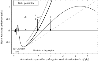
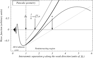
Figure 1: Cut through the function $r\psi(\vec{r})$ in a confined geometry for a van der Waals interaction with scattering length $a=3\,\beta_{6}$ , where $\beta_{6}=\left(\frac{2\mu C_{6}}{\hbar^{2}}\right)^{1/4}$ is the van der Waals length. We have chosen $a=3\beta_{6}$ as an illustrative value; for comparison, $a\approx 0.6\,\beta_{6}$ for ${}^{87}\textrm{Rb}$, $a\approx-10\,\beta_{6}$ for ${}^{133}\textrm{Cs}$, and $a>4\,\beta_{6}$ for ${}^{86}\textrm{Sr}$. Left panel: function $z\psi(\rho=0,z)$ as a function of $z$ for 2D confinement (tube) with $\sigma=1.95\,\beta_{6}$. Right panel: function $\rho\psi(\rho,z=0)$ as a function of $\rho$ for 1D confinement (pancake) with $\sigma=1.18\,\beta_{6}$. In both panels, the $s$-wave component of the solution to the free-space scattering problem at energy $E=\hbar^{2}k^{2}/2\mu$ is represented as a thin black line. For $r>\beta_{6}$ it has the asymptotic form corresponding to Eq. (7). The thick black line represents the 1D or 2D wave function in the noninteracting region obtained from Eq. (4) or (5). It is determined by a matching procedure with the free-space scattering wave function, as explained in the text. The previous theories Olshanii (1998); Petrov et al. (2000b) were based on a matching with the solution to free-space scattering at zero energy (dotted line), which has the asymptotic form corresponding to Eq. (8) for $r>\beta_{6}$. The resulting noninteracting 1D and 2D wave functions are represented by thick grey lines. They do not connect to the zero-energy wave function for the considered confinements. The lengths $\beta_{6}$, $a$ and $1/k$ are indicated by arrows.

Any scattering solution $\psi(\vec{r})$ of Eq. (1) is composed of an incident wave and a scattered wave. A plane wave basis can be used for the incident wave, and the scattered wave can be expressed with the noninteracting Green’s function $G(\vec{r},\vec{r}^{\prime})$ of the system for $U(r)=0$. Namely, for 2D confinement, one has:

$$\psi(\vec{r})\;=\;\phi_{nm}(\vec{\rho})e^{iq_{nm}z}-\int G_{2D}(\vec{r},\vec{r}^{\prime})U(r^{\prime})\psi(\vec{r}^{\prime})d^{3}\vec{r}^{\prime}$$ (2)

where $\phi_{nm}(\vec{\rho})$ denotes the unit-normalised 2D isotropic harmonic oscillator eigenstate of principal quantum number $n$ and angular quantum number $m$, and $q_{nm}=\sqrt{\frac{2\mu}{\hbar^{2}}E-(2n+1+|m|)/\sigma^{2}}$ is the wave number of the incident plane wave. The Green’s function reads:

$$G_{2D}(\vec{r},\vec{r}^{\prime})=\sum_{\nu,\mu}\!\phi_{\nu\mu}(\vec{\rho})\phi_{\nu\mu}(\vec{\rho})\frac{e^{iq_{\nu\mu}|z-z^{\prime}|}}{2iq_{\nu\mu}}$$

For 1D confinement, one has:

$$\psi(\vec{r})\;=\;\varphi_{n}(z)e^{i\vec{q}_{n}\cdot\vec{\rho}}-\int G_{1D}(\vec{r},\vec{r}^{\prime})U(r^{\prime})\psi(\vec{r}^{\prime})d^{3}\vec{r}^{\prime}$$ (3)

where $\varphi_{n}(z)$ denotes the unit-normalised 1D harmonic oscillator eigenstate of vibrational index $n$, and $\vec{q}_{n}$ is the wave vector of the incident plane wave with norm $q_{n}=\sqrt{\frac{2\mu}{\hbar^{2}}E-(n+\frac{1}{2})/\sigma^{2}}$ . The Green’s function reads:

$$G_{1D}(\vec{r},\vec{r}^{\prime})=\sum_{\nu}\varphi_{\nu}(z)\varphi_{\nu}(z^{\prime})\frac{i}{4}H_{0}^{(1)}(q_{\nu}|\rho-\rho^{\prime}|)$$

where $H_{\alpha}^{(1)}$ is the first Hankel function.

We first assume that the interaction potential $U(r)$ has a finite range $r_{b}$. This means that there is a separation $r_{0}\gg r_{b}$ beyond which the wave function is essentially a solution of Eq. (1) with $U(r)=0$, that is to say a solution of the noninteracting problem. This is indeed the case for typical atomic interactions which drop off as $-C_{6}/r^{6}$van der Waals potentials. Because of this fast drop-off, the wave function (at sufficiently low energy) reaches its noninteracting form for $r^{4}\gg\frac{1}{20}\beta_{6}^{4}$, where $\beta_{6}=\left(\frac{2\mu C_{6}}{\hbar^{2}}\right)^{1/4}$ Julienne (1996). The separation $r_{0}$ is therefore on the order of $\beta_{6}$, which ranges typically from 2 nm to 5 nm.

We further assume that the interaction potential $U$ scatters only $s$ waves. The scattering of partial waves of arbitrary order under cylindrical confinement was treated in detail in Ref. Kim et al. (2005). Retaining only $s$-wave scattering is valid in the absence of shape resonances and if the cold-collision condition $kr_{0}<1$ is satisfied, where $\hbar k=\sqrt{2\mu E}/\hbar$ is the collisional momentum (see Appendix).

Under these two assumptions, the noninteracting form of Eqs (2-3) is obtained by first taking the limit $r\gg r^{\prime}$ of the Green’s function (since $r>r_{0}\gg r_{b}\sim r^{\prime}$) and then approximating the remaining integral over $\vec{r}^{\prime}$ by $\phi_{\nu,\mu}(0)$ (or $\varphi_{\nu}(0)$) times a quantity $4\pi A$ which does not depend on the indices $\nu$ or $\mu$ appearing inside the Green’s funtion (taking into account the dependence on $\nu,\mu$ would introduce higher-order partial wave scattering Kim et al. (2005) - see Appendix). These two steps are formally equivalent to taking the Green’s function out of the integral in Eqs. (2-3) and evaluate it at $r^{\prime}=0$. Note that this can be achieved at any $r$ by replacing the potential $U(r)$ by a regularised contact interaction Fermi (1934). For 2D confinement, one finds Petrov and Shlyapnikov (2001)

$$\psi(\vec{r})\;\mathop{=}_{r>r_{0}}\phi_{nm}(\vec{\rho})e^{iq_{nm}z}-4\pi A_{nm}\sum_{\nu,\mu}\!\phi_{\nu\mu}(\vec{\rho})\phi_{\nu\mu}(0)\frac{e^{iq_{\nu\mu}|z|}}{2iq_{\nu\mu}}$$ (4)

and for 1D confinement Olshanii (1998),

$$\psi(\vec{r})\;\mathop{=}_{r>r_{0}}\varphi_{n}(z)e^{i\vec{q}_{n}\cdot\vec{\rho}}-4\pi A_{n}\sum_{\nu}\varphi_{\nu}(z)\varphi_{\nu}(0)\frac{i}{4}H_{0}^{(1)}(q_{\nu}\rho)$$ (5)

wher the factors $A_{mn}$ and $A_{n}$ are to be determined.

The wave function $\psi$ can also be expanded in spherical partial waves:

$$\psi(\vec{r})=\sum_{\ell=0}^{\infty}\sum_{m=-\ell}^{\ell}\psi_{\ell,m}(r)Y_{\ell,m}(\theta,\varphi)$$ (6)

where $Y_{\ell,m}$ are the spherical harmonics and $\theta$ the angle between $\vec{r}$ and the $z$ axis, $\varphi$ the angle between $\vec{\rho}$ and the $x$ axis. At short separations, the confining potential $V(\vec{r})$ is negligible, so one can expect that within a certain range $r_{1}$ related to the confinement length $\sigma$ (see Appendix), the wave function is close to a solution of Eq. (1) with $V(\vec{r})=0$, that is to say, a solution of the free-space scattering problem. Beyond $r_{0}$, the partial waves of this solution reach their noninteracting form which is known to be a combination of regular and irregular spherical Bessel functions. Consistent with the $s$-wave approximation, there is no irregular Bessel function for $\ell\neq 0$, ie no scattered partial wave. For the $s$ wave $(\ell=0)$, we have:

$$\psi_{00}(r)=\eta\left(\frac{\sin kr}{kr}-a(k)\frac{\cos kr}{r}\right)\quad\textrm{for }r_{0}<r<r_{1},$$ (7)

where $\eta$ is a normalisation factor to be determined and $a(k)=-\tan\delta_{k}/k$ is the energy-dependent s-wave scattering length introduced in Refs. Blume and Greene (2002); Bolda et al. (2002) ($\delta_{k}$ is the usual $s$-wave phase shift, related to the $s$-wave component of the reactance matrix $K_{s}(k)=-\tan\delta_{k}$). This energy-dependent scattering length contains all the effects of the interaction on the wave function in the region $r_{0}<r<r_{1}$, and for any collisional energy $E$. For moderately tight traps $\sigma\gg r_{0}$ leading to small collisional energies, there is a range of $r$ for which Eq. (7) simplifies to:

$$\psi(\mathbf{r})=\eta\left(1-\frac{a}{r}\right)$$ (8)

where $a=\lim_{k\to 0}a(k)$ is the scattering length of the potential. However, for very tight lattices, $\sigma$ may be close to $r_{0}$ and only Eq. (7) holds.

Figure 2: The 1D interaction strength (left panel) and the 2D interaction strength (right panel) in dimensionless units as a function of the ratio of the 3D scattering length $a$ over the confinement dimension $\sigma$ ($a$ is varied and $\sigma$ is fixed). As in Fig. 1, $\sigma=1.95\,\beta_{6}$ in left panel and $\sigma=1.18\,\beta_{6}$ in the right panel. The dots are obtained by numerically solving the problem of two atoms interacting through a Lennard-Jones potential in a 3D cylindrically-symmetric trap; dots in the left panel (tube geometry) were taken from Ref. Bergeman et al. (2003) and confirmed by us, while we calculated the dots in right panel (pancake geometry) using the adaptive grid refinement method of Ref. Mitchell and Tiesinga (2005). The dashed curves correspond to the formulæ (9) and (10) with the zero-energy scattering length $a$, and the solid curves corresponds to the same formulæ using the energy-dependent scattering length $a(k)$ instead of $a$. Here, $a(k)$ has been calculated in the effective-range approximation, Eq. (11), which is valid almost everywhere except for small positive scattering lengths where the approximation causes a spurious resonance.

The essence of the method used in Refs. Olshanii (1998) and Petrov and Shlyapnikov (2001) is to assume that $\sigma\gg r_{0}$ and match the noninteracting expressions (4) and (5), respectively, with the free-space expression (8) in the region $r_{0}<r<r_{1}$ where they are both valid. (In Ref. Olshanii (1998), this is implicitly achieved by use of a 3D regularised contact interaction). By performing the matching procedure up to zeroth order in the asymptotic expansion in $r/\sigma$ near $r=0$, they obtain two relations yielding the two unknown factors $\eta$ and $A_{nm}$ (or $A_{n}$). From that knowledge, they deduce the effective 1D and 2D interaction strengths in the quasi-1D or 2D regime ($q_{n},q_{nm}\ll k$):

$$g_{1D} = \frac{\hbar^{2}}{\mu\sigma}\left(\frac{\sigma}{a}+\frac{\zeta(1/2)}{\sqrt{2}}\right)^{-1}$$ (9)

$$g_{2D} = 4\pi\frac{\hbar^{2}}{\mu}\left(\frac{\sqrt{2\pi}\sigma}{a}+\ln\left(\frac{B}{\pi q_{0}^{2}\sigma^{2}}\right)\right)^{-1}$$ (10)

with $B\approx 0.915$ and $\zeta(1/2)/\sqrt{2}\approx-1.033$, where $\zeta$ is the Riemann zeta function. The singularity in these expressions as a function $a$, $\sigma$, or $q_{0}$ corresponds to the confinement-induced resonance. Note, however, that these analytical formulæ are valid only when $\sigma$ is large with respect to $r_{0}$.

We stress here that the method can be extended by matching the $s$-wave component of the noninteracting expressions (4) or (5) with the more general free-space expression (7). It is straightforward to see that a matching to zeroth order in $r/\sigma$ results in the same conditions as those of Refs. Petrov and Shlyapnikov (2001); Olshanii (1998), but with the scattering length $a$ being replaced by the energy-dependent $a(k)$ in all the formulæ. In particular, $a$ is replaced by $a(k)$ in the expressions for $\eta$, $A_{nm}$, $A_{n}$, and Eqs. (9-10). Surprisingly, we find that once the two unknown factors $\eta$ and $A_{nm}$ (or $A_{n}$) are determined this way, the expression (4) or (5) match the expression (7) up to second order in $r/\sigma$, $ie$ the next two orders automatically match without the need for extra parameters. This was checked numerically both in 2D and 1D confinement, and we give in the Appendix an analytical derivation of this result for 2D confinement, based on mathematical assumptions which we checked numerically. As a result, the expressions (4) or (5) and (7) can be matched within less than 1% for $\sigma\gtrsim r_{0}$. In Fig. 1 we illustrate the matching of the wave functions for a confinement $\sigma$ close to $r_{0}$, in the case of a van der Waals interaction $U(r)=-\frac{C_{6}}{r^{6}}$, for which $r_{0}\approx\beta_{6}$, as stated earlier. The figure shows both the $s$-wave component of the solution to the 3D free-space problem (which is highly oscillatory for $r<r_{0}$, and has the asymptotic form (7) for $r>r_{0}$) and the noninteracting wave function along either the $z$ or $\rho$ directions. For better comparison, we should plot only the $s$-wave component of the noninteracting wave function, but this happens to be very slowly converging numerically. The inclusion of higher-order partial waves thus induces a second-order difference (because $\psi_{2,m}(r)\propto r^{2}$ for small $r$), but one can still appreciate the very good matching of the two functions even at these extreme confinements. In contrast, the two functions calculated from the original theory do not match.

The fact that we can gain two orders in the matching procedure by using the free-space expression (7) implies that the replacement $a\to a(k)$ greatly improves the accuracy and the range of validity of the original theory. Although we do not have an estimation of the accuracy on $g_{1}$ and $g_{2}$, we expect the extended theory to give reasonnably good predictions for $\sigma\gtrsim r_{0}$. This improvement brought by the simple replacement $a\to a(k)$ not so surprising in view of the results reported in Refs. Bolda et al. (2002); Blume and Greene (2002); Bolda et al. (2003); Stock et al. (2005); Idziaszek and Calarco (2006), which have shown the relevance of energy-dependent scattering lengths for the accurate calculation of energy levels in 3D confined geometries. It has been long known in other contexts that contact interaction models are significantly improved when the coupling constants are proportional to the energy-dependent scattering length (or reactance matrix) Masnou-Seeuws (1982) . Similar extensions of (9) and (10) were considered in Refs. Wouters et al. (2003); Granger and Blume (2004); Yurovsky (2005) in order to take into account the energy dependence due to a scattering resonance at low energy. In Ref. Yurovsky (2005), a renormalised contact interaction was used, leading to the replacement of $a$ by the quantity $\frac{2\mu}{4\pi\hbar^{2}}T(k)$, where $T(k)=\frac{4\pi\hbar^{2}}{2\mu}a(k)(1+ika(k))^{-1}$ is the $T$-matrix. This complex quantity is equivalent to the real $a(k)$ at low energy. Here we focus on the energy dependence for strong confinement even in the absence of any resonance.

In the quasi-1D ($q_{nm}\ll k$) or quasi-2D ($q_{n}\ll k$) regimes, the collisional energy is set by the confinement length $\sigma$ and can be relatively high, although the effective collisions in the weak directions are cold. An interesting consequence of the extended theory is that if the confinement is strong enough, the collisional energy can probe the energy-dependence of $a(k)$. For a standard contact potential Fermi (1934), $a(k)$ is constant and equal to $a$. However, a more realistic $a(k)$ has some energy dependence. For instance, in the effective-range approximation, $a(k)$ has the resonant form:

$$a(k)\approx\frac{a}{1-\frac{1}{2}k^{2}ar_{e}},$$ (11)

where $r_{e}$ is the effective range of the potential Bethe (1949). This approximation works well for short-range interactions with a large scattering length $a\gg r_{e}$. In the case of van der Waals interactions, the effective range $r_{e}$ is a simple function of $a$ and $\beta_{6}$ Flambaum et al. (1999); Gao (1998):

$$r_{e}=\frac{2}{3}\frac{\beta_{6}^{2}}{\bar{a}}\left(\left(\frac{\bar{a}}{a}\right)^{2}+\left(\frac{\bar{a}}{a}-1\right)^{2}\right)$$ (12)

where $\bar{a}=2\pi\beta_{6}/\Gamma(1/4)^{2}$. More elaborate analytical expressions of $a(k)$ valid for any $a$ have been derived for van der Waals interactions Gao (1998). The interest of Eqs. (11) and (12) is that they give a simple two-parameter description of the collisions for a wide range of energies.

To illustrate these ideas, we calculated the 1D interaction strength $g_{1D}$ for a van der Waals interaction consistent with the Lennard-Jones parameters of the numerical calculation reported in Ref. Bergeman et al. (2003). The authors observed a difference between their numerical calculation and the analytic formula (9) where $a$ is taken as the zero-energy scattering length. They suggested that this difference comes the fact that the confinement-induced resonance in $g_{1D}$ results from a Feshbach resonance with a trap bound state, whose binding energy is not predicted accurately by a pseudopotential based only on the scattering length. As a result, the formula (9) does not predict the resonance at the right location. However, we show in Fig. 2 that the same formula used in conjunction with the replacement $a\to a(k)$ in the effective range approximation reproduces the numerical calculations very well. This is because the effective range approximation is able to reproduce the binding energy of the last bound state accurately. The only region where the effective range approximation fails is for small scattering lengths $a\ll\beta_{6}$, where it predicts a spurious resonance, as visible in Fig. 2.

We also calculated the 2D interaction strength and checked that a similar situation occurs in the pancake configuration. Using the adaptive grid refinement method of Ref. Mitchell and Tiesinga (2005), we solved the Schrödinger equation (1) for a Lennard-Jones interaction $U(r)=\frac{C_{12}}{r^{12}}-\frac{C_{6}}{r^{6}}$ and a cylindrical harmonic trap. The tight pancake limit is obtained by setting the ratio of axial and radial frequencies to 400 (thus leading to a spatial aspect ratio of 1/20), and the tight confinement scale is set to $\sigma=1.18\,\beta_{6}$. The parameter $C_{12}$ is adjusted to set the number of bound states supported by the interaction and the scattering length. From this calculation, we obtained the eigenenergies and then used Eq. (21) of Ref. Busch et al. (1998) to extract the 2D scattering length. We found that it shows very little dependence on the number of bound states, which can be as low as 2, saving computational efforts. Using Eq. (7) of Ref. Petrov and Shlyapnikov (2001) (or Eq. (15) of Ref. Lee et al. (2002)), we could then relate the 2D scattering length to the interaction strength $g_{2D}$ for any $q_{0}$ - we chose a $q_{0}$ given by the zero-point momentum in the weak direction. Figure (2) compares this numerical $g_{2D}$ with the analytical formula (9) for the same $q_{0}$. Again, the position of the confinement-induced resonance for negative scattering lengths Petrov et al. (2000b) is correctly predicted by (9) provided the energy-dependent scattering length is used. As previously, the effective range approximation works well, except for small scattering lengths. These results also suggest that the observation of the resonance may provide useful information about the effective range of the interaction.

In summary, we have shown that the effective 1D or 2D interactions of ultracold bosons in strongly confined systems are governed by 3D collisions at a relatively high energy determined by the confinement. The effect of these high-energy collisions can be well described by a single quantity, the energy-dependent scattering length, up to extremely tight confinements. For van der Waals interactions, this quantity itself can be expressed in the effective range approximation in terms of the zero-energy scattering length and the van der Waals length. This parametrized energy-dependent scattering length leads to an accurate analytic prediction of the confinement-induced resonance both in 1D and 2D confinements.

Appendix

In this appendix, we show that for 2D confinement the matching procedure is effective up to second order in the expansion in $r/\sigma$ near $r=0$. Without loss of generality, we take the wave function to be symmetric around the $z$ axis ($ie$ $m=0$ in Eq. (4)), so that Eq. (6) can be written as

$$\psi(\vec{r})=\sum_{\ell=0}^{\infty}\psi_{\ell}(r)i^{\ell}(2\ell+1)P_{\ell}(\cos\theta)$$ (13)

where $P_{\ell}(x)$ is the Legendre polynomial. The basic approximation is to assume that the components $\psi_{\ell}$ are proportional to those of the free-space solution. With the assumption that only the $s$-wave component is scattered by the potential, we set:

$$\psi_{0}(r) {\displaystyle\mathop{=}_{r>r_{0}}} \eta_{0}\phi_{n0}(0)\big{(}j_{0}(kr)+ka(k)y_{0}(kr)\big{)}$$ (14)

$$\psi_{\ell\neq 0}(r) {\displaystyle\mathop{=}_{r>r_{0}}} \eta_{\ell}\phi_{n0}(0)\,j_{\ell}(kr)$$ (15)

where $j_{\ell}$ and $y_{\ell}$ are the spherical Bessel functions, and $\eta_{\ell}$ are factors to be determined. (Note that with this definition, $\eta$ in Eq. (7) is equal to $\eta_{0}\phi_{n0}(0)$). Since only components of even $\ell$ are coupled to the $s$-wave component by the trapping potential $V(\vec{r})$, we can discard odd-$\ell$ components (they do not play a role in the scattering process). An expansion near $r=0$ of Eq. (13) therefore reads

$$\phi_{n0}(0)\left[\eta_{0}\left(-\frac{ka(k)}{kr}+1\right)+\left(\eta_{0}\frac{ka(k)}{2}\right)kr-\left(\frac{\eta_{0}}{6}+\frac{\eta_{2}}{3}P_{2}(\cos\theta)\right)(kr)^{2}-\left(\eta_{0}\frac{ka(k)}{24}\right)(kr)^{3}+\dots\right]$$ (16)

This is to be matched with Eq. (4). Using the explicit form of the harmonic oscillator solutions $\phi_{n0}$, it can be written as

$$\phi_{n0}(0)\Upsilon_{n}\left[\frac{\rho}{\sqrt{2}\sigma},\,\frac{z}{\sqrt{2}\sigma},\,-\frac{1}{2}q_{00}^{2}\sigma^{2}\right]$$ (17)

with

$$\Upsilon_{n}\left[u,\,v,\,\epsilon\right] = e^{-\frac{u^{2}}{2}}L_{n}(u^{2})\cosh(2v\sqrt{n+\epsilon})-\frac{A_{n0}}{\sqrt{2}\sigma}\Lambda\left[u,v,\epsilon\right]$$

$$\Lambda\left[u,\,v,\,\epsilon\right] = \sum_{\nu=0}^{\infty}\frac{e^{-2v\sqrt{\nu+\epsilon}}}{\sqrt{\nu+\epsilon}}e^{-\frac{u^{2}}{2}}L_{\nu}(v^{2})$$

where the $L_{\nu}$ is the Laguerre polynomial. For Eq. (17) a partial wave expansion appears not feasible, so we resort to evaluating the expressions along the $\rho$ and $z$ axes. Along the $z$ axis ($\rho=0$), we find the following expansion

$$\Lambda[0,v,\epsilon] = \frac{1}{v}+\zeta(\!\!\begin{array}[]{c}\frac{1}{2}\!\end{array},\epsilon)+(2\epsilon-1)v+2\zeta(\!-\begin{array}[]{c}\!\frac{1}{2}\end{array},\epsilon)v^{2}$$ (21)

$$+\frac{1}{6}\left[(2\epsilon-1)^{2}-\frac{1}{3}\right]v^{3}+\dots$$

Along the $\rho$ axis ($z=0$), we find the following expansion

$$\Lambda[u,0,\epsilon] = \frac{1}{u}+\zeta(\begin{array}[]{c}\!\!\frac{1}{2}\!\end{array},\epsilon)+(2\epsilon-1)u$$ (27)

$$+\left[\frac{1}{2}(2\epsilon-1)\zeta(\begin{array}[]{c}\!\!\frac{1}{2}\!\end{array},\epsilon)-\zeta(\!-\begin{array}[]{c}\!\frac{1}{2}\end{array},\epsilon)\right]u^{2}$$

$$+\frac{1}{6}\left[(2\epsilon-1)^{2}+\frac{2}{3}\right]u^{3}+\dots$$

In these expansions, $\zeta$ refers to the Hurwitz zeta function which we define as follows

$$\zeta(s,\epsilon)=\lim_{N\to\infty}\sum_{n=0}^{N}\frac{1}{(n+\epsilon)^{s}}-\frac{(N+\epsilon+\frac{1}{2})^{-s+1}}{-s+1}$$

for $-1<s<1$, generalizing the definition given in Refs. Bergeman et al. (2003); Moore et al. (2004). The first expansion (21) was found using the counter-term method explained in these references with the refined counter term $\int_{0}^{N+\frac{1}{2}+\epsilon}\frac{\exp(-2\sqrt{s}x)}{\sqrt{s}}ds$. The second expansion (27) was guessed from the expected result (16), and checked numerically. Because of the very slow convergence of the sum in $\Lambda[u,0,\epsilon]$ , we could not check the terms directly. Instead, we noted that the Laplace transform of $\Lambda$ with respect to the argument $u$ is related to the Lerch transcendent $\Phi$ Erdélyi et al. (1953):

$$\int_{0}^{\infty}e^{-su}\Lambda[u,0,\epsilon]du=\frac{1}{s+\frac{1}{2}}\Phi\left(\frac{s-\frac{1}{2}}{s+\frac{1}{2}},\frac{1}{2},\epsilon\right)$$

and assumed there is a direct correspondence between the Laplace transform of the terms in (27) and the terms in the asymptotic expansion of the Laplace transform near $s\to\infty$.

Matching the expressions (16) and (17) along the $z$ direction leads to the following relations for each order of the expansion:

$$\eta_{0}a(k) = A_{n0}$$ (28)

$$\eta_{0} = 1-\frac{A_{n0}}{\sqrt{2}\sigma}\zeta(\begin{array}[]{c}\!\!\frac{1}{2}\!\end{array},\epsilon)$$ (30)

$$\eta_{0}\frac{k^{2}a(k)}{2} = \frac{A_{n0}}{2\sigma^{2}}(k^{2}\sigma^{2})$$ (31)

$$\left(\frac{\eta_{0}}{6}+\frac{\eta_{2}}{3}\right)\!\!k^{2} = \!\frac{k^{2}}{2}-\frac{1+2n}{2\sigma^{2}}+\!\frac{A_{n0}}{\sqrt{2}\sigma^{3}}\zeta(\begin{array}[]{c}\!\!-\frac{1}{2}\!\end{array},\epsilon)$$ (33)

$$\eta_{0}\frac{ka(k)}{24}k^{3} = \frac{A_{n0}}{24\sigma^{4}}\left(k^{4}\sigma^{4}-\frac{1}{3}\right)$$ (34)

while, matching along the $\rho$ direction leads to the following relations

$$\eta_{0}a(k) = A_{n0}$$ (35)

$$\eta_{0} = 1-\frac{A_{n0}}{\sqrt{2}\sigma}\zeta(\begin{array}[]{c}\!\!\frac{1}{2}\!\end{array},\epsilon)$$ (37)

$$\eta_{0}\frac{k^{2}a(k)}{2} = -\frac{A_{n0}}{2\sigma^{2}}(k^{2}\sigma^{2})$$ (38)

$$\left(\frac{\eta_{0}}{6}-\frac{\eta_{2}}{6}\right)\!\!k^{2} = \frac{1+2n}{4\sigma^{2}}$$ (42)

$$-\frac{A_{n0}}{2\sqrt{2}\sigma^{3}}\left[\frac{k^{2}\sigma^{2}}{2}\zeta(\begin{array}[]{c}\!\!\frac{1}{2}\!\end{array},\epsilon)+\zeta(\!-\begin{array}[]{c}\!\frac{1}{2}\end{array},\epsilon)\right]$$

$$\eta_{0}\frac{ka(k)}{24}k^{3} = \frac{A_{n0}}{24\sigma^{4}}\left(k^{4}\sigma^{4}+\frac{2}{3}\right)$$ (43)

where we make use of $2\epsilon-1=-k^{2}\sigma^{2}$. Relations (28-30) and (35-37) are the same and determine $A_{n0}$ and the $s$-wave factor:

$$\eta_{0}=\frac{1}{1+\frac{a(k)}{\sqrt{2}\sigma}\zeta(\begin{array}[]{c}\!\!\frac{1}{2}\!\end{array},-\frac{q_{00}^{2}\sigma^{2}}{2})}$$ (44)

Relations (31) and (38) are the same and are both satisfied with the previous determination of $A_{n0}$ and $\eta_{0}$. Relations (33) and (42) are consistent and give the same determination of the $d$-wave factor:

$$\eta_{2}=\eta_{0}\left(\frac{3a(k)}{\sqrt{2}k^{2}\sigma^{3}}\zeta(\!-\begin{array}[]{c}\!\frac{1}{2}\end{array},-\!\!\begin{array}[]{c}\frac{q_{00}^{2}\sigma^{2}}{2}\end{array}\!\!)-\frac{1}{2}\right)+\frac{3}{2}\frac{q_{n0}^{2}}{k^{2}}$$ (45)

However, neither relation (34) or (43) are satisfied with the previous determination of $A_{n0}$ and $\eta_{0}$ (because of the terms $-\frac{1}{3}$ and $\frac{2}{3}$), which means that the free-space approximation (14-15) is valid up to order $r^{2}$. The error is $\phi_{n0}(0)|\eta_{0}a(k)|\frac{1}{24\sigma^{4}}r^{3}$. The range of $r$ for which this error is negligible determines the range $[r_{0},r_{1}]$ where a matching is possible. Since the error increases with $r$, we can define $r_{1}$ as the $r$ for which the ratio between the error and the wave function (16) is equal to a certain tolerance $\alpha$. In the limit of large scattering lengths, one finds

$$r_{1}=(24\alpha)^{1/4}\sigma.$$

The range [$r_{0},r_{1}$] where the two functions can be matched to within the tolerance $\alpha$ exists as long as $r_{1}>r_{0}$, ie

$$\sigma>(24\alpha)^{-1/4}r_{0}.$$ (46)

For instance, for $\alpha=1\%$, one gets $\sigma>1.43r_{0}.$ This indicates that the method works even for a confinement length $\sigma$ on the order of the range $r_{0}$.

We can also check that this is consistent with our assumption that only $s$ waves are scattered. Higher-order partial wave scattering arises if we take into account the dependence of $A_{n0}$ on $\nu$. The first correction is $A_{n0}\to A_{n0}+(\nu+\frac{1}{2})B_{n0}$, and leads to the term $B_{n0}\sigma^{2}/z^{3}$ along the $z$ axis. This term is to be matched with the leading-order term of the scattered $d$-wave term $(-K_{2})\eta_{2}\phi_{n0}(0)y_{2}(kz)(-5)P_{2}(\cos 0)$, where $K_{2}$ is the $d$-wave reactance matrix element. In the absence of shape resonance, $K_{2}$ is purely determined by the long-range van der Waals behaviour of the interaction, $K_{2}\approx-\frac{1}{100}(k\beta_{6})^{4}$ - see Eq. (8) of Ref. Gao (1998). This leads to:

$$B_{n0}=-\eta_{2}\frac{\sigma}{20}\frac{(k\beta_{6})^{4}}{(k\sigma)^{3}}$$

$d$-wave scattering is negligible if $|B_{n0}|\ll|A_{n0}|$. In the quasi-1D regime ($q_{n0}\ll k$ and $k\sim 1/\sigma$), and using the value of $\eta_{2}$ (45), one finds:

$$\sigma^{4}\gg\left(\frac{1}{40}|1-\sigma/a(k)|\right)\beta_{6}^{4},$$

which for a wide range of scattering lengths is consistent with the condition (46) and the cold collision condition $kr_{0}<1$ given in the text.

References

- Görlitz et al. (2001) A. Görlitz, J. M. Vogels, A. E. Leanhardt, C. Raman, T. L. Gustavson, J. R. Abo-Shaeer, A. P. Chikkatur, S. Gupta, S. Inouye, T. Rosenband, et al., Phys. Rev. Lett. 87, 130402 (2001).
- Denschlag et al. (2002) J. H. Denschlag, J. E. Simsarian, H. Häffner, C. McKenzie, A. Browaeys, D. Cho, K. Helmerson, S. L. Rolston, and W. D. Phillips, J. Phys. B 35, 3095 (2002).
- Richard et al. (2003) S. Richard, F. Gerbier, J. H. Thywissen, M. Hugbart, P. Bouyer, and A. Aspect, Phys. Rev. Lett. 91, 010405 (2003).
- Spielman et al. (2006) I. B. Spielman, P. R. Johnson, J. H. Huckans, C. D. Fertig, S. L. Rolston, W. D. Phillips, and J. V. Porto, Phys. Rev. A 73, 020702 (2006).
- Ido and Katori (2003) T. Ido and H. Katori, Phys. Rev. Lett. 91, 053001 (2003).
- Ludlow et al. (2006) A. D. Ludlow, M. M. Boyd, T. Zelevinsky, S. M. Foreman, S. Blatt, M. Notcutt, T. Ido, and J. Ye, Phys. Rev. Lett. 96, 033003 (2006).
- Olshanii (1998) M. Olshanii, Phys. Rev. Lett. 81, 938 (1998).
- Petrov et al. (2000a) D. S. Petrov, G. Shlyapnikov, and J. T. M. Walraven, Phys. Rev. Lett. 85, 3745 (2000a).
- Paredes et al. (2004) B. Paredes, A. Widera, V. Murg, O. Mandel, S. Fölling, I. Cirac, G. V. Shlyapnikov, T. W. Hänsch, and I. Bloch, Nature 429, 277 (2004).
- Kinoshita et al. (2004) T. Kinoshita, T. Wenger, and D. S. Weiss, Science 305, 1125 (2004).
- Petrov et al. (2000b) D. S. Petrov, M. Holzmann, and G. V. Shlyapnikov, Phys. Rev. Lett. 84, 2551 (2000b).
- Tiesinga et al. (2000) E. Tiesinga, C. J. Williams, F. H. Mies, and P. S. Julienne, Phys. Rev. A 61, 063416 (2000).
- Blume and Greene (2002) D. Blume and C. H. Greene, Phys. Rev. A 65, 043613 (2002).
- Bergeman et al. (2003) T. Bergeman, M. G. Moore, and M. Olshanii, Phys. Rev. Lett. 91, 163201 (2003).
- Bolda et al. (2002) E. L. Bolda, E. Tiesinga, and P. S. Julienne, Phys. Rev. A 66, 013403 (2002).
- Julienne (1996) P. S. Julienne, J. Res. Natl. Inst. Stand. Technol. 101, 487 (1996).
- Kim et al. (2005) J. I. Kim, J. Schmiedmayer, and P. Schmelcher, Phys. Rev. A 72, 042711 (2005).
- Fermi (1934) E. Fermi, Nuovo Cim. 11, 157 (1934).
- Petrov and Shlyapnikov (2001) D. S. Petrov and G. V. Shlyapnikov, Phys. Rev. A 64, 012706 (2001).
- Mitchell and Tiesinga (2005) W. F. Mitchell and E. Tiesinga, Appl. Num. Math. 52, 235 (2005).
- Bolda et al. (2003) E. L. Bolda, E. Tiesinga, and P. S. Julienne, Phys. Rev. A 68, 032702 (2003).
- Stock et al. (2005) R. Stock, A. Silberfarb, E. L. Bolda, and I. H. Deutsch, Phys. Rev. Lett. 94, 023202 (2005).
- Idziaszek and Calarco (2006) Z. Idziaszek and T. Calarco, quant-phys/0604205 (2006).
- Masnou-Seeuws (1982) F. Masnou-Seeuws, J. Phys. B 15, 883 (1982).
- Wouters et al. (2003) M. Wouters, J. Tempere, and J. T. Devreese, Phys. Rev. A 68, 053603 (2003).
- Granger and Blume (2004) B. E. Granger and D. Blume, Phys. Rev. Lett. 92, 133202 (2004).
- Yurovsky (2005) V. A. Yurovsky, Phys. Rev. A 71, 012709 (2005).
- Bethe (1949) H. A. Bethe, Phys. Rev. 76, 38 (1949).
- Flambaum et al. (1999) V. V. Flambaum, G. F. Gribakin, and C. Harabati, Phys. Rev. A 59, 1998 (1999).
- Gao (1998) B. Gao, Phys. Rev. A 58, 4222 (1998).
- Busch et al. (1998) T. Busch, B.-G. Englert, K. Rza̧żewski, and M. Wilkens, Found. of Phys. 28, 549 (1998).
- Lee et al. (2002) M. D. Lee, S. A. Morgan, M. J. Davis, and K. Burnett, Phys. Rev. A 65, 043617 (2002).
- Moore et al. (2004) M. G. Moore, T. Bergeman, and M. Olshanii, J. Phys. IV France 116, 69 (2004), cond-mat/0210556.
- Erdélyi et al. (1953) A. Erdélyi, W. Magnus, F. Oberhettinger, and F. G. Tricomi, Higher Transcendental Functions, vol. 1 (McGraw Hill, New York, 1953).