Weighted Assortative And Disassortative Networks Model

Abstract

Real-world networks process structured connections since they have non-trivial vertex degree correlation and clustering. Here we propose a toy model of structure formation in real-world weighted network. In our model, a network evolves by topological growth as well as by weight change. In addition, we introduce the weighted assortativity coefficient, which generalizes the assortativity coefficient of a topological network, to measure the tendency of having a high-weighted link between two vertices of similar degrees. Network generated by our model exhibits scale-free behavior with a tunable exponent. Besides, a few non-trivial features found in real-world networks are reproduced by varying the parameter ruling the speed of weight evolution. Most importantly, by studying the weighted assortativity coefficient, we found that both topologically assortative and disassortative networks generated by our model are in fact weighted assortative.

I Introduction

There is a wave of interest to study complex networks by statistical physical means review1 ; review2 ; review3 . The area of studies include the Internet internet ; internet2 ; internet3 , the World-Wide Web www , scientific collaboration networks (SCN) scn ; scn2 , biological networks bio ; bio2 and the world-wide airport network (WAN) airport . In all these cases, one can naturally identify the subject under study with a graph. For instance, an airport in a WAN can be represented by a vertex; and there is a link between two vertices if and only if there is a direct flight between the corresponding airports. Although these complex networks are drawn from vastly different systems in the real world, they exhibit the following universal properties:

1. Scale-free behavior of degree distribution: Let $P(k)$ be the probability that any vertex is connected to $k$ other vertices (i.e. the vertex is of degree $k$). In many real-world networks, $P(k)\sim k^{-\gamma}$ with $2\lesssim\gamma\lesssim 3$ powerlawk .

2. Clustering property: Clustering of a vertex $c_{i}$ gives the probability that two nearest neighbors are connected with each other. And the average clustering coefficient $C=\sum_{i}c_{i}/N$, where $N$ is the number of vertices in the network, measures the global density of interconnected vertex triplets in the network. Real-world networks in general exhibit higher clustering coefficient than those in random networks smallworld .

3. Small-world property: A network is said to have small-world property if the average shortest path length between two vertices scales at most logarithmically with $N$ for fixed mean degree smallworld ; smallworld2 .

4. Correlations of degree: An assortative (A disassortative) network tends to connect vertices with similar (dissimilar) degrees. Previous studies found that social networks tend to be assortative while technological and biological networks are generally disassortative cor .

Various network models have been proposed to simulate or explain the properties found in complex networks in the real world. For instance, the Erdös-Rényi random graph model random1 ; random2 generates static networks that exhibit small-world property. Nonetheless, the degree distribution of the network generated is Poissonian rather than a power-law. Later on, Barabási and Albert (BA) extended the Erdös-Rényi random graph model by evolving the network using a linear preferential attachment mechanism powerlawk . The ideas behind the BA model are that most real-world networks tend to growth with time, and a new vertex tends to connect to pre-existing high-degree vertices. Sen further incorporated non-linear growth property of the number of links to the BA model by demanding the number of links of the vertex added at time $t$ to be $t^{\theta}$ for some positive constant $\theta$ acc . Both the BA model and the Sen model generate networks with scale-free topology; but they failed to reproduce the degree correlations and clustering properties of real-world networks.

Structural organization of a network can be characterized by degree-dependent average nearest-neighbors degree $k_{\text{nn}}(k)$ internet , the degree-dependent average clustering coefficient $C(k)$ c(k) and assortativity coefficient $r$ r . Pan et al. proposed the generalized local-world models xli in which a subset of vertices is randomly chosen every time step. The newly added vertex can only make connection to vertices in this subset. Moreover, Liu et al. proposed the self-learning mutual selection model jliu in which every vertex has some probability to self evolve in each time step. These two models successfully reproduce the $k_{\text{nn}}(k)$, $C(k)$ and $r$ observed in real-world networks. However, these quantities only depend on the topological structure of a network. The relative importance between different links is not taken into consideration. To provide a better description of a network, the intensity of interaction among vertices should be taken into account. One may define the weight of a link $w_{ij}$ as the intensity of interaction between vertices $i$ and $j$, and the vertex strength $s_{i}$ as the sum of weight of the links connected to $i$:

$$s_{i}=\sum_{j\in\Gamma(i)}w_{ij}~{},$$ (1)

where $\Gamma(i)$ denotes the nearest neighbors of $i$. For instance, the weight $w_{ij}$ in WAN refers to the number of seats available on the direct flight connections between the airports $i$ and $j$. And $s_{i}$ represents the total traffic going through the airport $i$. To probe the weighted networks’ architecture, a set of weighted quantities are introduced, such as the weighted degree-dependent average clustering coefficient $C^{w}(k)$ and the weighted degree-dependent average nearest-neighbor degree $k^{w}_{\text{nn}}(k)$ powerlaws . However, no one has proposed a quantity that can directly measure the correlations of degree with inclusion of weight so far. Here we introduce the weighted assortativity coefficient $r^{w}$ to measure the tendency of having a high-weighted link between two vertices of similar degrees. In addition, we propose a model that incorporates the essential features of strength preferential attachment, nonlinear growth of number of links, and weight evolution of existing links. We call this the Weight Evolution Model. The rule of weight evolution are based on the notion that “the rich always gets richer”. In other words, high-weighted link has higher probability to evolve. Besides, inspired by the work of Dorogovtsev and Mendes dm , existing links in the graph can be removed. By altering the speed of weight evolution, our model can generate both assortative and disassortative networks with scale-free behavior and non-trivial clustering properties. Most importantly, both topologically assortative and disassortative networks generated by our model are in fact weighted assortative.

In Section II, we define the Weight Evolution Model. We report our analytical calculations and numerical results on the probability distributions of strength of vertex and weight of link in Section III. Then in Section IV we define the weighted assortativity coefficient and compare the organizational structure found in real-world networks with our numerical simulations. Finally, we give a brief summary in Section V.

II Weight Evolution Model

The model starts with a small number $N_{0}$ of fully connected undirected vertices. The weight of all the $N_{0}(N_{0}-1)/2$ initial links are set to $w_{0}$. In each time step, the network evolves under the following rules:

1. Topological growth: A new vertex is added to the network. We assume that the number of links of the new vertex is an increasing function of the network size. Specifically, a vertex with $\left[pt^{\theta}\right]$ links are added to the network at time $t$ for some fixed constants $p>0$ and $0<\theta<1$. (Here $[x]$ denotes the value of $x$ rounded to the nearest integer.) These $\left[pt^{\theta}\right]$ links are all of weight $w_{0}$ and are randomly connected to the existing vertices according to the strength preferential probability $\Lambda_{i}$, which is defined as weighted1 ; weighted2

   $$\Lambda_{i}=\frac{s_{i}}{\sum_{j}s_{j}}~{}.$$ (2)

2. Evolution of weight: The link between vertices $i$ and $j$ is chosen to evolve with probability $Q_{i,j}$ proportional to its weight, namely

   $$Q_{i,j}=\frac{w_{ij}}{\sum_{a<b}w_{ab}}~{}.$$ (3)

   The weight will update according to the equation

   $$w_{ij}\longrightarrow w_{ij}+\text{sgn}(q)~{},$$ (4)

   where

   $$\text{sgn}(q)=\left\{\begin{array}[]{cl}1&\text{if~{}}q>0~{},\\ -1&\text{if~{}}q<0~{},\\ 0&\text{if~{}}q=0~{}.\end{array}\right.$$ (5)

   At time step $t$, this process will repeat $\left[|q|t^{\theta}\right]$ times and a link is removed if the weight equals to $0$. (In other words, the sign of $q$ determines the addition or subtraction of weight of a link; and the magnitude of $q$ specifies the rate of the addition/subtraction per time step.)

Note that $p$, $q$ and $\theta$ are the tunable parameters in this model.

Clearly, our model generalizes the BA model powerlawk and the Sen model acc . In particular, our model is reduced to the BA model by setting $\theta=0$, $q=0$, $w_{0}=1$, and reduced to the Sen model by setting $0\leq\theta\leq 1$, $p=1$, $q=0$ and $w_{0}=1$.

We now justify the validity of our rules. Note that in most real-world networks, new vertices are introduced one at a time; and they tend to connect to the pre-existing high strength vertices. In the example of WAN, new airport tends to establish flights to existing airports with heavy traffic. Our topological growth process is used to capture this kind of network growth. Moreover, our weight evolution mechanism models the trend that the link with higher weight have a higher probability to evolve. For instance, in SCN powerlaws , a vertex represent a scientist and a link is present if two scientists have co-authored at least one paper. The weight between two scientists is higher if they have higher number of co-authored papers. Naturally, if the weight between two scientists is high, the probability for them to collaborate again is also high.

III Strength and weight

In our model, the processes of topological growth and weight evolution are Markovian. Thus, the evolution of our network can be calculated accurately by mean field approximation. Appendix A reports the mean field calculation of the probability distribution of vertex strength $P(s)$ and probability distribution of weight of link $P(w)$. We found that $P(s)\sim s^{-\gamma_{s}}$ and $P(w)\sim w^{-\gamma_{w}}$, where

$$\gamma_{s}=1-\left[\frac{2(w_{0}p+q)}{(\theta-1)w_{0}p-2q}\right]~{},$$ (6)

$$\gamma_{w}=1+\left[\frac{w_{0}p+q}{(\theta+1)q}\right]~{}.$$ (7)

To check the validity of our analytical solution, we performed numerical simulations on our network model for different values of $q$ and $\theta$. Since $p$, $q$ and $w_{0}$ govern the relative speed between new link addition and weight evolution, one can fix two of these three parameters without losing any generality. In this paper, we fix $p=1$ and $w_{0}=10$ unless otherwise stated. Besides, we set the number of initial vertices $N_{0}$ to $5$; and we have checked that the networks generated using different values of $p$ and $N_{0}$ exhibit similar behaviors as long as $N_{0}\ll N$. Using this set of parameters, we found that statistical data collected from the network equilibrate after $t\gtrsim 5\,000$. Hence, we collect all our statistical data at $t=10\,000$ and all the data reported here have been averaged over 50 independent runs. Our model successfully reproduces the scale-free behavior of the probability distributions of strength and weight with a tunable exponent that depends on the microscopic mechanism ruling the weight evolution. We found in Appendix B that the numerical simulation results agree with the mean field approximation.

IV Clustering and correlations

In this section, we first discuss the quantities used to characterize the clustering and correlations behaviors of a network. Then we introduce the weighted assortativity coefficient $r^{w}$. Finally, we report the numerical simulation results of our model.

IV.1 Quantities Characterizing A Weighted Network

We overload the notation by labeling the vertex added to the network in time step $i$ also by $i$. The clustering of $i$ is defined as

$$c_{i}=\frac{1}{k_{i}(k_{i}-1)}\sum_{j,h}a_{ij}a_{ih}a_{jh}~{},$$ (8)

where $k_{i}$ is the degree of $i$ and

$$a_{ij}=\left\{\begin{array}[]{cl}1&\text{if a link exist between $i$ and $j$}~{},\\ 0&\text{if there is no link between $i$ and $j$}~{}.\end{array}\right.$$ (9)

If vertex $i$ has less than two neighbors, $c_{i}$ is set to $0$. Clustering $c_{i}$ measures the local cohesiveness of vertex $i$ while the average clustering coefficient $C=\sum_{i}c_{i}/N$ measures the global density of interconnected triples in the network. Organizational structure of network can be further studied via the degree-dependent average clustering coefficient $C(k)$,

$$C(k)=\frac{1}{NP(k)}\sum_{i:k_{i}=k}c_{i}~{},$$ (10)

which is the mean clustering for vertices with degree $k$.

To have a better understanding of the organizational structure of weighted networks, the weighted clustering $c^{w}_{i}$ is introduced and defined as powerlaws

$$c^{w}_{i}=\frac{1}{s_{i}(k_{i}-1)}\sum_{j,h}\frac{(w_{ij}+w_{ih})}{2}a_{ij}a_{ih}a_{jh}~{},$$ (11)

If vertex $i$ tends to form triples with other vertices by its’ high-weighted links, then $c^{w}_{i}>c_{i}$ meaning that the topological clustering of $i$ underrates the cohesiveness of $i$. The weighted average clustering coefficient $C^{w}$ and weighted degree-dependent average clustering coefficient $C^{w}(k)$ are defined as the average of $c^{w}_{i}$ over all vertices and over all vertices with degree $k$, respectively powerlaws .

The degree correlation is another important information of the network. Recall that the network is said to be assortative if the vertices tend to connect to other vertices which have similar (dissimilar) properties. Newman introduced the assortativity coefficient r ; cor

$$r=\frac{M^{-1}\sum_{\phi}(\prod_{i\in F(\phi)}k_{i})-[\frac{M^{-1}}{2}\sum_{\phi}(\sum_{i\in F(\phi)}k_{i})]^{2}}{\frac{M^{-1}}{2}\sum_{\phi}(\sum_{i\in F(\phi)}k_{i}^{2})-[\frac{M^{-1}}{2}\sum_{\phi}(\sum_{i\in F(\phi)}k_{i})]^{2}}$$ (12)

to measure the degree correlation between linked vertices, where $F(\phi)$ denotes the set of the two vertices connected by the $\phi$th link and $M$ is the total number of links in the network. This measure $r$ is positive (negative) for assortative (disassortative) networks; and $r=0$ for a random graph. Note that $r$ is independent of the weight of each link of a network.

To probe the degree correlation of the network, one may also study the average nearest-neighbors degree, which is defined as internet

$$k_{\text{nn},i}=\frac{1}{k_{i}}\sum_{j\in\Gamma(i)}k_{j}.$$ (13)

The degree-dependent average nearest-neighbors degree $k_{\text{nn}}(k)$ is the mean of $k_{\text{nn},i}$ restricted to the class of degree $k$ vertices. In an assortative (disassortative) network, vertices with high degree tend to connect to other vertices with high (low) degree, thus $k_{\text{nn}}(k)$ would be an increasing (decreasing) function of $k$. In real-world weighted networks, high degree vertices could connect to small degree vertices with low weight, while connect to high degree vertices with high weight. For instance, in WAN, the high degree airport $i$ could have a lot of direct flight to another high degree airport $j$, while have less number of flight to a low degree airport $h$. In this case, $k_{\text{nn}}(k)$ will underestimate the tendency for having heavy traffic between two similar degree airports. To handle this problem, Barrat et al. proposed the weighted average nearest-neighbor degree powerlaws

$$k^{w}_{\text{nn},i}=\frac{1}{s_{i}}\sum_{j\in\Gamma(i)}w_{ij}k_{j}.$$ (14)

If the weighted degree-dependent nearest-neighbors degree $k^{w}_{\text{nn}}(k)$ is an increasing function of $k$, similar degree vertices tend to link together. Besides, the weights of these links tend to be high. Consequently, the network is weighted assortative.

Although one can figure out that the network is assortative or disassortative if $k^{w}_{\text{nn}}(k)$ is increasing or decreasing with $k$, a quantity directly describing the weighted assortativity is needed. Thus we introduce the weighted assortativity coefficient

$$r^{w}=\frac{H^{-1}\sum_{\phi}(\varpi_{\phi}\prod_{i\in F(\phi)}k_{i})-[\frac{H^{-1}}{2}\sum_{\phi}(\varpi_{\phi}\sum_{i\in F(\phi)}k_{i})]^{2}}{\frac{H^{-1}}{2}\sum_{\phi}(\varpi_{\phi}\sum_{i\in F(\phi)}k_{i}^{2})-[\frac{H^{-1}}{2}\sum_{\phi}(\varpi_{\phi}\sum_{i\in F(\phi)}k_{i})]^{2}}~{},$$ (15)

where $\varpi_{i}$ is the weight of the $\phi$th link, $F(\phi)$ is the set of the two vertices connected by the $\phi$th link and $H$ is the total weight of all links in the network. Just like $r$, $r^{w}$ lies between $-1$ and $1$. Moreover, $r^{w}$ is positive for weighted assortative networks, while negative for weighted disassortative networks. If $r^{w}>r$, a high-weighted link tend to connect two similar degree vertices together. In fact, $r^{w}$ reduces to $r$ if all weights in the network are equal. Furthermore, $r^{w}=r=0$ for a random graph. Fig. 1 illustrates that the values of $r$ and $r^{w}$ of a network can differ greatly. The network in Fig. 1 consists of two complete graphs of three vertices that are joined together by a highly weighted link. Since the five out of seven of the links in this network connect two vertices of different degree together, the assortativity coefficient $r$ of this network is negative. (In fact $r=-1/6$.) On the other hand, the weighted assortativity coefficient $r^{w}$ of this network is positive. This can be understood as follows. The link between the two degree three vertices in this network carries the most weight. So after coarse-graining, the network is similar to the one making up of a single link connecting two degree one vertices together plus another four isolated vertices. And clearly, the coarse-grained network is assortative. Therefore, when the weight of link are taken into account, the network in Fig. 1 ought to be assortative rather than disassortative. (In fact $r^{w}=2/3$.) In this respect, the weighted assortativity coefficient $r^{w}$ better determines the assortativity of networks with weighted links than the assortativity coefficient $r$.

Figure 1: A network whose $r<0$ but $r^{w}>0$.

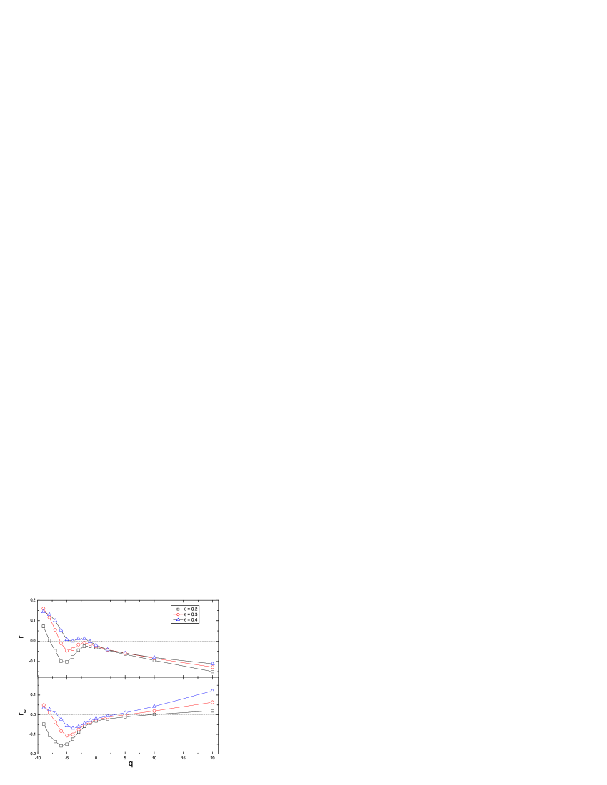
Figure 2: Assortativity coefficient $r$ and weighted assortativity coefficient $r^{w}$ versus $q$ for various $\theta$. The statistics taken right at time $t=10\,000$. And we have averaged over $50$ independent runs in all the data reported here. All error bars are $\lesssim 10^{-2}$.

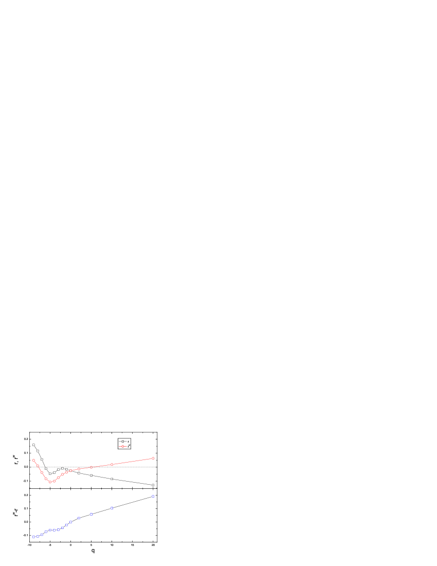
Figure 3: The comparison between $r$ and $r^{w}$ for $\theta=0.3$.

IV.2 Simulation Results

As shown in Fig. 2, our model can generate assortative networks ($r>0$), such as those found in social networks, when $q\ll 0$. Our model can also generate disassortative networks ($r<0$), such as those found in technological networks, when $q\gg 0$. Surprisingly, $r^{w}>0$ for both assortative and disassortative networks provided that $|q|\gtrsim 7$. This observation indicates that the topological assortativity coefficient underrates the contributions of high-weighted links between similar degree vertices. Our finding shows that studying the assortativity of a network by considering network topology alone r ; cor does not give a complete picture of the organizational structure of the network.

The difference between $r^{w}$ and $r$ (Fig. 3) can be understood qualitatively by considering the evolution mechanisms of our model. For $q\gg 0$, a newly added vertex is the one with low degree and it tends to connect to existing high-strength and high-degree vertices. This process leads to topologically disassortative behavior. Meanwhile, a link introduced at an early time, which connects two old vertices having similar degrees together, tends to be high-weighted as $q>0$. This leads to the observed weighted assortative behavior. On the other hand, assortative networks emerge at $q\ll 0$. It is because the strength of old vertices are low. Hence, there is a high chance for two young vertices having similar degrees to connect. As $\theta$ increases, the strength of old vertices decrease while the new vertices enter the network with a higher strength. Thus, for $q\ll 0$, the value of $|q|$ required for the emergence of assortative behavior decreases with $\theta$. This is precisely what we have observed in Fig. 2.

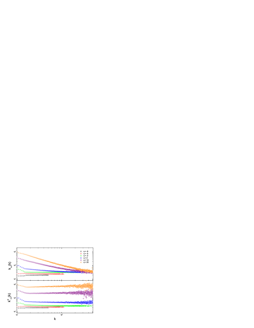
Figure 4: $k_{\text{nn}}(k)$ and $k^{w}_{\text{nn}}(k)$ for various $q$ for $\theta=0.3$.

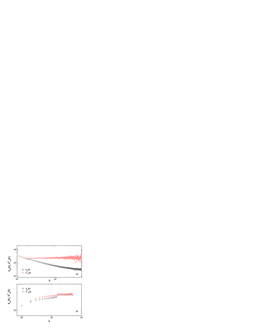
Figure 5: Comparison of $k_{\text{nn}}(k)$ and $k^{w}_{\text{nn}}(k)$ for (a) $q=10$ and (b) $q=-9$ for $\theta=0.3$.

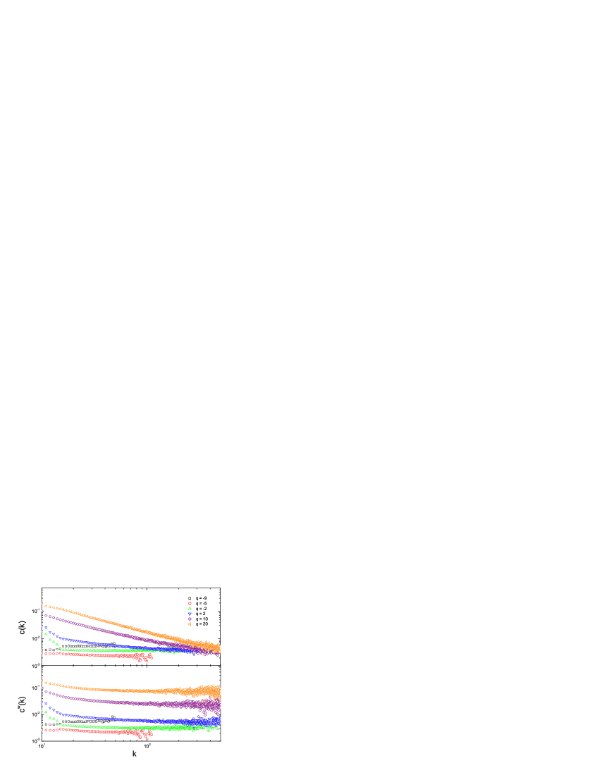
Figure 6: $C(k)$ and $C^{w}(k)$ for various $q$ for $\theta=0.3$.

As shown in Fig. 4, $k_{\text{nn}}(k)$ exhibits decreasing power-law behavior for $q\gg 0$, indicating that the networks are disassortative. For $q\ll 0$, $k_{\text{nn}}(k)$ is a gently increasing function of $k$. It is worth noting that in some empirical studies of real-world networks powerlaws , both $k_{\text{nn}}(k)$ and $k^{w}_{\text{nn}}(k)$ show assortative behavior with $k^{w}_{\text{nn}}(k)>k_{\text{nn}}(k)$. As shown in Fig. 5, our model successfully reproduces these important features. Remarkably, $r^{w}<r$ while $k^{w}_{\text{nn}}(k)>k_{\text{nn}}(k)$ for $q\ll 0$. This points out that it is difficult to compare the weighted assortativity and topological assortativity by studying the difference between $k^{w}_{\text{nn}}(k)$ and $k_{\text{nn}}(k)$.

Two types of $C(k)$ are found in real-world networks c(k) ; class . In the first type, $C(k)$ does not exhibit strong dependency on $k$. While in the second type, $C(k)$ shows a decreasing power law spectrum. Fig. 6 clearly shows that our model can reproduce both kinds of features. In particular, $C(k)$ is flat for $q\ll 0$ and it becomes a decreasing power law for $q\gg 0$. Moreover, $C^{w}(k)$ is larger than $C(k)$, especially at large $k$, which is a feature found in real-world networks powerlaws . This result indicates that the topological clustering coefficient $C(k)$ underestimate the cohesiveness of the network. It is because $C(k)$ cannot tell us whether large degree vertices tend to form interconnected triples with its’ high-weighted links.

V Conclusions

In summary, we have introduced the Weight Evolution Model which couples dynamical evolution of weight with topological network growth. We have also introduced the weighted assortativity coefficient $r^{w}$ to characterize the degree correlation of a weighted network. Our model reproduced many features found in real-world networks, such as scale-free behavior, assortative and disassortative behavior, and two types of clustering structures. Most importantly, both topologically disassortative and assortative networks are regarded as weighted assortative if the weight of links is taken into account, indicating that the topological assortativity coefficient $r$ underrates the contributions of high-weighted links between similar degree vertices. This result may give us some idea for why social networks are found to be assortative, while technological networks and biological networks show an opposite behavior in previous studies r ; cor . It is instructive to investigate if all real-world networks can be regarded as weighted assortative.

Appendix A Analytical calculations of strength and weight

Recall that initially the network is a complete graph of $N_{0}$ vertices. And in each time step a new vertex is added. There are two ways to alter the strength of an existing vertex $i$: (a) $i$ is connected to the newly added vertex $j$ with probability $\Lambda_{i}$ given by Eq. (2), or (b) the weight of the link between $i$ and one of its neighboring vertices evolves according to Eqs. (3)–(5).

By mean field approximation and by treating all discrete variables as continuous, the strength $s_{i}$ of the vertex added at time $i$ satisfies

$$\frac{ds_{i}(t)}{dt} = w_{0}pt^{\theta}\frac{s_{i}(t)}{\sum_{\ell}s_{\ell}(t)}+qt^{\theta}\frac{\sum_{j\in\Gamma(i)}w_{ij}(t)}{\sum_{a<b}w_{ab}(t)}$$ (16)

$$= w_{0}pt^{\theta}\frac{s_{i}(t)}{\sum_{\ell}s_{\ell}(t)}+2qt^{\theta}\frac{s_{i}(t)}{\sum_{\ell}s_{\ell}(t)}~{},$$

for $t>i$. Note that the first and second terms represent the strength change due to topological growth and evolution of weight, respectively.

Since the total strength of the network increases $2(w_{0}p+q)t^{\theta}$ approximately in each time step,

$$\sum_{l}s_{l}(t)\approx\int_{0}^{t}2(w_{0}p+q)t^{\theta}dt=\frac{2(w_{0}p+q)}{\theta+1}\,t^{\theta+1}~{}.$$ (17)

Putting Eq. (17) into Eq. (16) and using the initial condition $s_{i}(t=i)=w_{0}[pi^{\theta}]$, we conclude that

$$s_{i}(t) \approx w_{0}pi^{\theta}\left(\frac{t}{i}\right)^{(\theta+1)(w_{0}p+2q)/2(w_{0}p+q)}$$ (18)

$$= w_{0}pt^{\theta}\left(\frac{t}{i}\right)^{[2q-(\theta-1)w_{0}p]/2(w_{0}p+q)}~{}.$$

Since one vertex is added to the network in each time step, the network size $N{\approx}t$. The probability distribution of vertex strength can be computed by

$$P(s)\approx\frac{1}{t}\int_{0}^{t}\delta(s-s_{j}(t))dj~{},$$ (19)

where $\delta(x)$ is the Dirac delta function. Combined with Eq. (18), we conclude that in the infinite network size limit, the mean field approximation give $P(s)\sim s^{-\gamma_{s}}$ for $\textrm{min}(s_{i}(t))\leq s\leq\textrm{max}(s_{i}(t))$, where

$$\gamma_{s}=1-\left[\frac{2(w_{0}p+q)}{(\theta-1)w_{0}p-2q}\right]~{}.$$ (20)

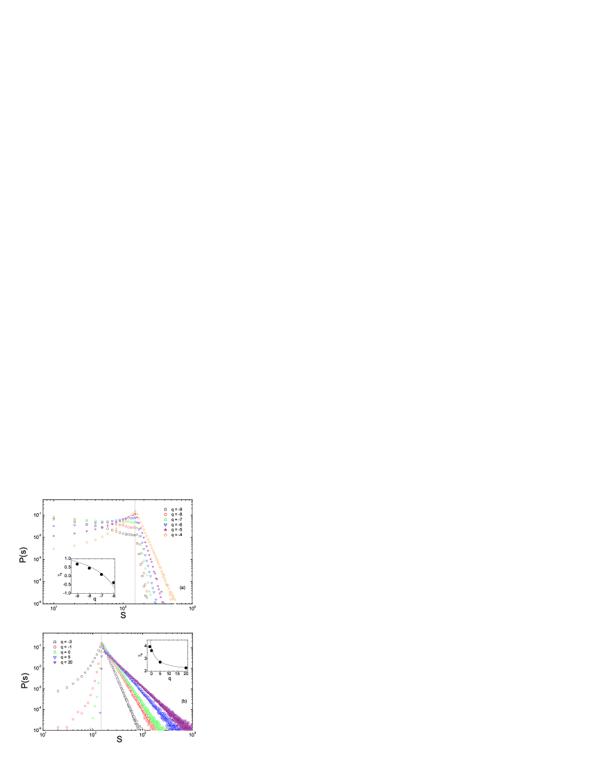
Figure 7: Probability distribution of strength $P(s)$ for $\theta=0.3$. A power-law function $P(s)\sim s^{-\gamma}$ is obtained in the range of (a) $s<s_{n}$ if $q<q_{c}=-3.5$ and (b) $s>s_{n}$ if $q>q_{c}$. The dashed line corresponds to $s=s_{n}=148$. The insert compares the values of $\gamma$ obtained from data fitting (filled circles) with the analytical solution $\gamma_{s}$ given by Eq. (20) (solid line).

The behavior of $P(s)$ can be classified according to the value of $q$:

1. If $q>q_{c}\equiv(\theta-1)w_{0}p/2$, Eq. (18) tells us that the degree of existing vertices are generally larger than the degree of the newly added vertex, i.e. $s_{i}(t)\geq s_{n}\equiv w_{0}pt^{\theta}$ for all $i$. Thus,

   $$P(s)\sim\left\{\begin{array}[]{lll}&0&\text{for~{}}s<s_{n}~{},\\ &s^{-\gamma_{s}}&\text{for~{}}s\geq s_{n}~{}.\end{array}\right.$$ (21)

   In particular, the network evolves purely by topological growth for $q=0$. And in this case, we find that $\gamma_{s}=(\theta-3)/(\theta-1)$ which is independent of $p$. Moreover, $\gamma_{s}\rightarrow 2$ as $q\rightarrow\infty$.

2. If $q=q_{c}$, $s_{i}(t)=s_{n}$ which is the same for all $i$. In this case, $P(s)$ is a delta function. In contrast, $P(s)$ is a delta function only when $\theta=1$ (i.e., when the network is fully connected) in the Sen model acc .

3. If $q<q_{c}$, $s_{i}(t)\leq s_{n}$ by Eq. (18). In other words, the newly added vertex have the highest strength. Using a similar argument as in the case of $q>q_{c}$, we found that the strength distribution $P(s)$ follows

   $$P(s)\sim\left\{\begin{array}[]{lll}&s^{-\gamma_{s}}&\text{for~{}}s<s_{n}~{},\\ &0&\text{for~{}}s\geq s_{n}~{}.\end{array}\right.$$ (22)

The evolution of weight can again be computed using mean field approximation. Therefore, we have

$$\frac{dw_{ij}(t)}{dt}\approx qt^{\theta}\frac{w_{ij}(t)}{\sum_{a<b}w_{ab}(t)}\approx\frac{(\theta+1)qw_{ij}(t)}{(w_{0}p+q)t}~{},$$ (23)

for $t>\max(i,j)$. Clearly, $w_{ij}(t)$ satisfies the initial condition $w_{ij}(t=\text{max}(i,j))=w_{0}$. Hence, we find

$$w_{ij}(t)\approx w_{0}\left[\frac{t}{\textrm{max}(i,j)}\right]^{(\theta+1)q/(w_{0}p+q)}~{}.$$ (24)

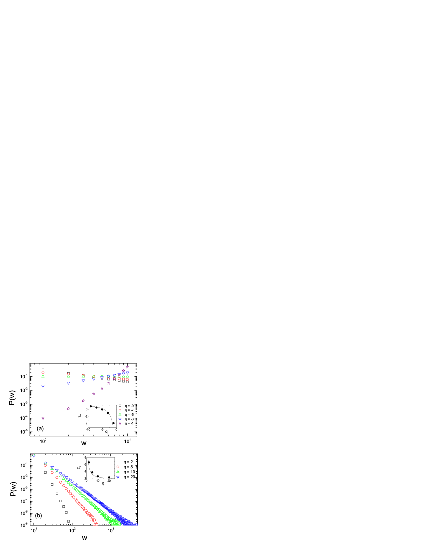
Figure 8: Probability distribution of weight $P(w)\sim w^{-\gamma_{w}}$ with (a) $q<0$ and (b) $q>0$. The insert compares the values of $\gamma_{w}$ obtained from data fitting (filled circles) and the mean field value given by Eq. (25) (solid line) for $\theta=0.3$.

In addition, the weight distribution $P(w)$, which gives the probability that a link with weight $w$, obeys $P(w)\sim w^{-\gamma_{w}}$ for $\textrm{min}(w_{ij})\leq w\leq\textrm{max}(w_{ij})$, where

$$\gamma_{w}=1+\left[\frac{w_{0}p+q}{(\theta+1)q}\right]~{}.$$ (25)

Appendix B Numerical results of probability distribution

Fig. 7 reports $P(s)$ obtained from numerical simulations for different values of $q$. It also compares the value of exponent obtained from fitting the numerically simulated data with the value predicted by analytical calculation. $P(s)$ follows a power-law function for $q\ll q_{c}$ or $q\gg q_{c}$ with exponent agree well with the value given by Eq. (20). Note that $P(s)$ is non-zero for $s>s_{n}$ when $q<q_{c}$ (Fig. 7(a)) and for $s<s_{n}$ when $q>q_{c}$ (Fig. 7(b)). This discrepancy is due to the fact that a small proportion of vertices evolves differently from the prediction of mean-field approximation. However, this value diminishes to zero rapidly and thus our analytical calculation remains valid. The weight probability distribution $P(w)$ for various $q$ is displayed in Fig. 8 along with the comparison between the fitted values of the exponent with the analytical predictions. For $q<0$, $w_{ij}\leq w_{0}$ for all links, so the power-law function is obtained for $w\leq w_{0}$ (Fig. 8(a)). For $q>0$, the power-law function is found to be in the range of $w\geq w_{0}$ (Fig. 8(b)).

References

- (1) S. N. Dorogovtsev and J. F. F. Mendes, Adv. Phys. 51, 1079 (2002).
- (2) R. Albert and A. L. Barabási, Rev. Mod. Phys. 74, 47 (2002).
- (3) M. E. J. Newman, SIAM Rev. 45, 167 (2003).
- (4) R. Pastor-Satorras, A. Vázquez, and A. Vespignani, Phys. Rev. Lett. 87, 258701 (2001).
- (5) A. Vázquez, R. Pastor-Satorras, and A. Vespignani, Phys. Rev. E 65, 066130 (2002).
- (6) R. Pastor-Satorras and A. Vespignani, Evolution and Structure of the Internet: A Statistical Physics Approach (Cambridge University Press, Cambridge, U.K., 2004).
- (7) R. Albert, H. Jeong, and A.-L. Barabási, Nature 401, 130 (1999).
- (8) M. E. J. Newman, Proc. Natl. Acad. Sci. U.S.A. 98, 404 (2001).
- (9) A.-L. Barabási, H. Jeong, Z. Néda, E. Ravasz, A. Schubert, and T. Vicsek, Physica A 311, 590 (2002).
- (10) H. Jeong, S. P. Mason, A.-L. Barabási and Z. N. Oltvai, Nature 411, 41 (2001).
- (11) E. Ravasz, A. L. Somera, D. A. Mongru, Z. N. Oltvai, and A.-L. Barabási, Science 297, 1551 (2002).
- (12) R. Guimerà, S. Mossa, A. Turtschi, and L. A. N. Amaral, Proc. Natl. Acad. Sci. U.S.A. 102, 7794 (2005).
- (13) A.-L. Barabási and R. Albert, Science 286, 509 (1999).
- (14) D. J. Watts and S. H. Strogatz, Nature 393, 440 (1998).
- (15) M. E. J. Newman, Phys. Rev. E 64, 016132 (2001).
- (16) M. E. J. Newman, Phys. Rev. E 67, 026126 (2003).
- (17) P. Erdös and A. Rényi. Publ. Math. (Debrecen) 6, 290 (1959).
- (18) B. Bollobás, Random Graphs (Academic Press, London, 1985), chap 2.
- (19) P. Sen, Phys. Rev. E. 69, 046107 (2004).
- (20) E. Ravasz and A.-L. Barabási, Phys. Rev. E 67, 026112 (2003).
- (21) M. E. J. Newman, Phys. Rev. Lett. 89, 208701 (2002).
- (22) Z. Pan, X. Li, and X. Wang, Phys. Rev. E 73, 056109 (2006).
- (23) J.-G. Liu, Y.-Z. Dang, W.-X. Wang, Z.-T. Wang, T. Zhou, B.-H. Wang, Q. Guo, Z.-G. Xuan, S.-H. Jiang and M.-W. Zhao, arXiv:physics/0512270 (2005).
- (24) A. Barrat, M. Barthélemy, R. Pastor-Satorras, and A. Vespignani, Proc. Natl. Acad. Sci. U.S.A. 101, 3747 (2004).
- (25) S. N. Dorogovtsev and J. F. F. Mendes, Europhys. Lett. 52, 33 (2000).
- (26) A. Barrat, M. Barthélemy, and A. Vespignani, Phys. Rev. Lett. 92, 228701 (2004).
- (27) A. Barrat, M. Barthélemy, and A. Vespignani, Phys. Rev. E. 70, 066149 (2004).
- (28) A. Vázquez, Phys. Rev. E. 67, 056104 (2003).