Circular and helical equilibrium solutions of inhomogeneous rods

Abstract

Real filaments are not perfectly homogeneous. Most of them have various materials composition and shapes making their stiffnesses not constant along the arclength. We investigate the existence of circular and helical equilibrium solutions of an intrinsically straight rod with varying bending and twisting stiffnesses, within the framework of the Kirchhoff model. The planar ring equilibrium solution only exists for a rod with a given form of variation of the bending stiffness. We show that the well known circular helix is not an equilibrium solution of the static Kirchhoff equations for a rod with non constant bending stiffness. Our results may provide an explanation for the variation of the curvature seen in small closed DNAs immersed in a solution containing Zn²⁺, and in the DNA wrapped around a nucleosome.

Instituto de Física, Universidade de São Paulo, USP
Rua do Matão, Travessa R 187, Cidade Universitária, 05508-900, São Paulo, Brazil

Keywords: Kirchhoff rod model, inhomogeneous rod, planar ring, generalized helices, planar elasticae, closed DNA

1 Introduction

Static and dynamics of one-dimensional structures have been the subject of intense research in Engineering, Physics and Biology. Such filamentary objects are present in both nature and man-made devices. The stability of sub-oceanic cables [1, 2], the tridimensional structure of biomolecules [3] and bacterial fibers [4], and the mechanical properties of nanosprings [5, 6, 7, 8] are few of many interesting problems investigated within elastic rod models.

In most cases, the rod is considered as having constant or uniform stiffness, but non-uniform rods have been considered in the literature. It has been shown that nonhomogeneous Kirchhoff rods may present spatial chaos [9, 10]. Domokos and Holmes studied buckled states of non-uniform elasticae [11]. Deviations from the helical structure of rods due to periodic variation of the Young’s modulus were verified numerically by da Fonseca, Malta and de Aguiar [12]. Homogeneous and nonhomogeneous rods subject to given boundary conditions were studied by da Fonseca and de Aguiar in [13]. The effects of a nonhomogeneous mass distribution in the dynamics of unstable closed rods have been analyzed by Fonseca and de Aguiar [14]. Goriely and McMillen [15] studied the dynamics of cracking whips [16], Kashimoto and Shiraishi [17] studied twisting waves in inhomogeneous rods, and Neuringer and Elishakoff [18] studied natural frequencies of inhomogeneous rods.

It is well known that straight, circular and helical rods are equilibrium solutions of the Kirchhoff model [19, 20, 21]. These solutions have been used to study the stability and buckling phenomena of loop elasticae [1, 22], the twist to writhe conversion phenomenon in twisted straight rods [23], and the stability of DNA configurations with or without self-contact [24], to name some examples.

Our aim here is to investigate the existence of circular and helical equilibrium solutions for an intrinsically straight, inextensible, unshearable, and inhomogeneous rod with circular cross-section, within the Kirchhoff rod model.

Establishing the stability (even in the case of simple equilibrium configurations) of a rod is a non-trivial task (see, for example, Refs. [22, 23, 24, 25, 26, 27, 28]). Since the study of the stability analysis departs from the knowledge of equilibrium solutions, our work is the starting point for the study of the stability of equilibrium solutions of inhomogeneous rods.

The inhomogeneity of the rod is considered through the bending and twisting coefficients varying along its arclength $s$, $B(s)$ and $C(s)$, respectively. We shall derive a set of non-linear differential equations for the curvature, $k_{F}(s)$, and the torsion, $\tau_{F}(s)$, of the centerline of an inhomogeneous rod, and then impose the necessary conditions to finding circular/helical solutions. Circular (ring) solutions have $k_{F}=$ Constant and $\tau_{F}=0$, while helical solutions have the curvature and torsion of the rod centerline satisfying the Lancret’s theorem: $k_{F}(s)/\tau_{F}(s)$ is constant [29, 30]. The well known circular helix is the particular case where both $k_{F}$ and $\tau_{F}$ are constant.

The fundamental theorem for space curves [30] states that the curvature and the torsion completely determine a space curve, but for its position in space. This is the reason for our choice of working with the curvature, $k_{F}(s)$, and the torsion, $\tau_{F}(s)$, of the rod centerline. We shall show that the solutions for $k_{F}(s)$ and $\tau_{F}(s)$ depend only on the bending coefficient, $B(s)$, an expected result since the centerline of the rod does not depend on the twisting coefficient (see for instance, Neukirch and Henderson [31]).

In Sec. II we present the static Kirchhoff equations for an intrinsically straight rod with circular cross section and varying stiffness, and derive the non-linear differential equations for the curvature and torsion of the rod. In Sec. III we analyse the cases of null torsion (straight and planar rods). We show that the ring solution of the static Kirchhoff equations only exists for a particular form of variation of the bending stiffness. In the case of twisted rods with varying bending stiffness, this ring solution is the only possible planar solution of the Kirchhoff equations. In the case of non-twisted rods, there exist other types of equilibrium planar solutions that depend on the bending stiffness. In Sec. IV we use the Lancret’s theorem for obtaining generalized helical solutions of the static Kirchhoff equations. We show that the circular helix is not an equilibrium solution of a rod that has non constant bending stiffness. We obtain generalized helical solutions that depend on the form of variation of the bending stiffness. As illustration, we compare the helical solution of a homogeneous rod with two types of helical solutions related to simple cases of inhomogeneous rods: (i) bending coefficient varying linearly, and (ii) bending varying periodically along the rod. In Sec. V we discuss the main results and possible applications to DNA.

2 The static Kirchhoff equations

The statics and dynamics of long, thin, inextensible and unshearable elastic rods are described by the Kirchhoff rod model. In this model, the rod is divided in segments of infinitesimal thickness to which the Newton’s second law for the linear and angular momenta are applied. We derive a set of partial differential equations (PDE) for the averaged forces and torques on each cross section and for a triad of vectors describing the shape of the rod. The set of PDE are completed with a linear constitutive relation between torque and twist.

The central axis of the rod, hereafter called centerline, is represented by a space curve ${\mathbf{x}}$ parametrized by the arclength $s$. We commonly describe a physical filament using a local basis, $\{{\mathbf{d}}_{1},{\mathbf{d}}_{2},{\mathbf{d}}_{3}\}$, which permits taking into account the twist deformation of the filament. This local basis is defined such that ${\mathbf{d}}_{3}$ is the vector tangent to the centerline of the rod (${\mathbf{d}}_{3}={\mathbf{t}}\equiv d{\mathbf{x}}/ds$), and ${\mathbf{d}}_{1}$ and ${\mathbf{d}}_{2}$ lie on the cross section plane. The local basis is related to the Frenet frame $\{{\mathbf{n}},{\mathbf{b}},{\mathbf{t}}\}$ of the centerline through

$$({\mathbf{d}}_{1}\;{\mathbf{d}}_{2}\;{\mathbf{d}}_{3})=({\mathbf{n}}\;{\mathbf{b}}\;{\mathbf{t}})\left(\begin{array}[]{ccc}\cos\xi&-\sin\xi&0\\ \sin\xi&\cos\xi&0\\ 0&0&1\end{array}\right)\;,$$ (1)

where the angle $\xi$ is the amount of twisting of the local basis with respect to ${\mathbf{t}}$.

We are interested in the equilibrium solutions of the Kirchhoff model, so our study departs from the static Kirchhoff equations [32]. For intrinsically straight isotropic rods, these equations are:

$$\mathbf{F}^{\prime}=0\;,$$ (2)

$$\mathbf{M}^{\prime}=\mathbf{F}\times\mathbf{d}_{3}\;,$$ (3)

$$\mathbf{M}=B(s)\,k_{1}\,\mathbf{d}_{1}+B(s)\,k_{2}\,\mathbf{d}_{2}+C(s)\,k_{3}\,\mathbf{d}_{3}\;,$$ (4)

where the following scaled variables were introduced:

$$s\rightarrow sL\;,\;\;\;\mathbf{F}\rightarrow\mathbf{F}\frac{EI}{L^{2}}\;,\;\;\;\mathbf{M}\rightarrow\mathbf{M}\frac{EI}{L}\;\;\;\mbox{and}\;\;\;k_{i}\rightarrow k_{i}\frac{1}{L}\;,i=1,2,3\;.$$ (5)

the vectors $\mathbf{F}$ and $\mathbf{M}$ are the resultant force and the corresponding moment with respect to the centerline of the rod, respectively, at a given cross section. The prime ^′ denotes differentiation with respect to $s$. $k_{i}$ are the components of the twist vector, $\mathbf{k}$, that controls the variations of the director basis along the rod through the relation

$${\mathbf{d}}^{\prime}_{i}={\mathbf{k}}\times{\mathbf{d}}_{i}\;,\;\;i=1,2,3\;.$$ (6)

$k_{1}$ and $k_{2}$ are related to the curvature of the centerline of the rod $(k_{F}=\sqrt{k^{2}_{1}+k^{2}_{2}})$ and $k_{3}$ is the twist density. $B(s)$ and $C(s)$ are the bending and twisting coefficients of the rod, respectively. Writing the force $\mathbf{F}$ in the director basis,

$${\bf{F}}=f_{1}{\bf{d}}_{1}+f_{2}{\bf{d}}_{2}+f_{3}{\bf{d}}_{3}\;,$$ (7)

the equations (2–4) give the following differential equations for the components of the force and twist vector:

$$f^{\prime}_{1}-f_{2}\,k_{3}+f_{3}\,k_{2}=0\;,$$ (8)

$$f^{\prime}_{2}+f_{1}\,k_{3}-f_{3}\,k_{1}=0\;,$$ (9)

$$f^{\prime}_{3}-f_{1}\,k_{2}+f_{2}\,k_{1}=0\;,$$ (10)

$$(B(s)\,k_{1})^{\prime}+(C(s)-B(s))\,k_{2}\,k_{3}-f_{2}=0\;,$$ (11)

$$(B(s)\,k_{2})^{\prime}-(C(s)-B(s))\,k_{1}\,k_{3}+f_{1}=0\;,$$ (12)

$$(C(s)\ k_{3})^{\prime}=0\;.$$ (13)

The equation (13) shows that the component $M_{3}=C(s)\,k_{3}$ of the moment in the director basis (also called torsional moment), is constant along the rod, consequently the twist density $k_{3}$ is inversely proportional to the twisting coefficient $C(s)$

$$k_{3}(s)=\frac{M_{3}}{C(s)}\;.$$ (14)

In order to look for circular (ring) and helical solutions of the Eqs. (8–13) the components of the twist vector $\mathbf{k}$ are expressed as follows:

$$k_{1} = k_{F}(s)\sin\xi\;,$$ (15)

$$k_{2} = k_{F}(s)\cos\xi\;,$$ (16)

$$k_{3} = \xi^{\prime}+\tau_{F}(s)\;,$$ (17)

where $k_{F}(s)$ and $\tau_{F}(s)$ are the curvature and torsion, respectively, of the rod centerline, and $\xi$ is given by Eq. (1).

Substituting Eqs. (15–17) in Eqs. (8–13), extracting $f_{1}$ and $f_{2}$ from Eqs. (12) and (11), respectively, differentiating them with respect to $s$, and substituting in Eqs. (8), (9) and (10), gives the following set of nonlinear differential equations:

$$[M_{3}\,k_{F}-B\,k_{F}\,\tau_{F}]^{\prime}-(B\,k_{F})^{\prime}\,\tau_{F}=0\;,$$ (18)

$$(B\,k_{F})^{\prime\prime}+k_{F}\,\tau_{F}[M_{3}-B\,\tau_{F}]-f_{3}\,k_{F}=0\;,$$ (19)

$$(B\,k_{F})^{\prime}\,k_{F}+f^{\prime}_{3}=0\;,$$ (20)

where we have omitted the dependence on $s$ to simplify the notation. Appendix A presents the details of the derivation of Eqs. (18–20).

The Eqs. (18–20) for the curvature, $k_{F}$, and torsion, $\tau_{F}$, do not depend on the twisting coefficient, $C(s)$. Therefore, the centerline of an inhomogeneous rod does not depend on the twisting coefficient unlike the case of homogeneous rods (see, for example, Eqs. (13) and (14) of Ref. [31]).

Langer and Singer [33] have obtained a set of first-order ordinary differential equations for the curvature and torsion of the centerline of a homogeneous rod that contains terms proportional to $k_{F}^{2}$ and $\tau^{2}_{F}$. The Eqs. (18–20) have the advantage of involving only terms linear in $k_{F}$ and $\tau_{F}$.

3 Planar solutions of inhomogeneous rods

Planar solutions are obtained by setting $\tau_{F}=0$ in Eqs. (18-20). The result is:

$$M_{3}\,k_{F}^{\prime}=0\;,$$ (21)

$$(B\,k_{F})^{\prime\prime}-f_{3}\,k_{F}=0\;,$$ (22)

$$(B\,k_{F})^{\prime}\,k_{F}+f^{\prime}_{3}=0\;,$$ (23)

Eq. (21) implies two different sets of solutions: $M_{3}\neq 0$ (twisted rods) and $M_{3}=0$ (non-twisted rods). Each case will be analysed separately.

3.1 Twisted rod: $M_{3}\neq 0$

As ($M_{3}\neq 0$), Eq. (21) leads to $k_{F}(s)=$ Constant $\equiv K$, which represents the circular solution (also known as planar ring solution). Eqs. (22) and (23) must be also satisfied, and their combination gives the following differential equation for the bending stiffness $B(s)$:

$$\frac{d}{ds}\left[B^{\prime\prime}+K^{2}B\right]=0\;,$$ (24)

or

$$B^{\prime\prime}+K^{2}B=\mbox{Constant }\equiv C_{0}\;,$$ (25)

where we have set $k_{F}=K$, and $C_{0}$ is a constant of integration. Therefore, the twisted ($M_{3}\neq 0$) ring solution of an inhomogeneous rod only exists if its bending stiffness satisfies the differential equation (25) (forced harmonic oscillator). The bending stiffness (solution of (25)) can be written in the form:

$$B(s)=A_{0}\cos(K\,s)+B_{0}\sin(K\,s)+C_{0}/K^{2}\;,$$ (26)

with $A_{0}$ and $B_{0}$ arbitrary constants.

Therefore, only an intrinsically straight inhomogeneous twisted rod ($M_{3}\neq 0$) with the bending stiffness given by Eq. (26), can display a planar ring configuration.

3.2 Non-twisted rod: $M_{3}=0$

In this case, Eq. (21) is automatically satisfied so the curvature $k_{F}(s)$ does not have to be constant.

From Eq. (22), we can obtain the following relation for $f_{3}(s)$:

$$f_{3}(s)=\frac{(Bk_{F})^{\prime\prime}}{k_{F}}\;.$$ (27)

Differentiating $f_{3}$ with respect to $s$ and substituting in Eq. (23), we obtain the following non-linear differential equation for the curvature $k_{F}(s)$:

$$k_{F}(Bk_{F})^{\prime\prime\prime}-k_{F}^{\prime}(Bk_{F})^{\prime\prime}+k_{F}^{3}(Bk_{F})^{\prime}=0\;.$$ (28)

If $k_{F}=$ Constant $\equiv K$ (the planar ring solution) the above equation gives the following differential equation for $B$:

$$\frac{d}{ds}\left[B^{\prime\prime}+K^{2}B\right]=0\;,$$ (29)

which is the same Eq. (24) and, therefore, gives the same condition for $B(s)$ shown in Eq. (26). In this case, $f_{3}(s)$ is given by:

$$f_{3}(s)=-K^{2}(A_{0}\cos Ks+B_{0}\sin Ks)\;.$$ (30)

So, the non-twisted planar ring ($k_{F}=$ Constant) is also an equilibrium solution of the static Kirchhoff equations if the bending stiffness of the inhomogeneous rod is given by Eq. (26).

Another solution of Eq. (28) for the curvature $k_{F}(s)$ comes from making $(Bk_{F})^{\prime}=0$, which gives

$$k_{F}(s)=\frac{\mbox{Constant}}{B(s)}\;,$$ (31)

and, from Eq. (27), $f_{3}(s)=0$.

It is a very interesting solution because it relates the curvature of the rod centerline to the bending stiffness. Also, the component of the force tangent to the rod centerline, $f_{3}$, is null for the set of solutions satisfying Eq. (31). In the particular case where $B(s)$ is given by Eq. (26), we can have two possible planar solutions: the planar ring $k_{F}(s)=K$, and the solution for which $k_{F}(s)$ is given by Eq. (31).

A kink is characterized by a piece of a filament having high curvature $k_{F}$ (or small radius of curvature, $R=1/k_{F}$). The Kirchhoff approach is not appropriate for modelling kinks in rods because in the derivation of the Kirchhoff equations it is assumed that the rod centerline radius of curvature is much larger than the cross-section radius [20]. However, Haijun and Zhong-can [34] used the Kirchhoff rod model to show that variations in the curvature of a closed rod may lead to instabilities responsible for the kink formation. Within the limits of validity of the Kirchhoff model, Eq. (31) shows that pieces of a rod with small bending coefficient may lead to equilibrium configurations with large curvature. Therefore, our results can help explaining the onset of formation of kinks, since variations in the curvature of a filament can be originated by variations in the bending stiffness along it (Eq. (31)). In Section V we comment on an application of this result to small closed DNAs. Figure 1 illustrates a planar equilibrium solution given by Eq. (31) in the case of a rod with periodic variation of its bending stiffness.

The straight rod ($k_{1}=0$, $k_{2}=0$) is a trivial solution of the static Kirchhoff equations, and is a particular case of planar solutions. In the inhomogeneous case, the twist density, $k_{3}$, of the straight rod is not constant. According to Eq. (14), for a given external torque, $M_{3}$, the twist is large for pieces of the rod where the twisting coefficient, $C$, is small. This result could help in determining the regions where plastic deformations or ruptures start to occur in rods subjected to large stresses.

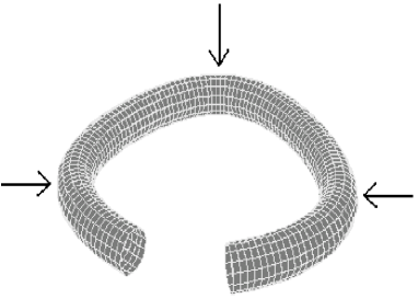
Figure 1: A non twisted planar solution of the Kirchhoff equations for a rod with periodic variation of the bending stiffness. The arrows point to the regions where the curvature is increased.

4 Helical solutions of inhomogeneous rods

In this section, we are considering the equilibrium solutions for the rod centerline in which $k_{F}\neq 0$ and $\tau_{F}\neq 0$. In order to find helical solutions for the static Kirchhoff equations, we apply the Lancret’s theorem to the equations (18–20). We first write the Lancret’s theorem in the form:

$$k_{F}(s)=\beta\,\tau_{F}(s)\;,$$ (32)

where $\beta\neq 0$ is a constant. Substituting Eq. (32) in Eq. (18) we obtain

$$\tau_{F}^{\prime}\,(M_{3}-B\,\tau_{F})-2\,\tau_{F}\,(B\,\tau_{F})^{\prime}=0\;.$$ (33)

Substituting Eq. (32) in Eq. (19) and extracting $f_{3}$, we obtain

$$f_{3}=\frac{(B\,\tau_{F})^{\prime\prime}}{\tau_{F}}+\tau_{F}\,(M_{3}-B\,\tau_{F})\;.$$ (34)

Differentiating $f_{3}$ with respect to $s$ and substituting in Eq. (20) we obtain the following differential equation for $\tau_{F}(s)$:

$$\frac{(B\,\tau_{F})^{\prime\prime\prime}}{\tau_{F}}-\frac{(B\,\tau_{F})^{\prime\prime}\tau_{F}^{\prime}}{\tau_{F}^{2}}+(\beta^{2}+1)\,\tau_{F}\,(B\,\tau_{F})^{\prime}=0\;,$$ (35)

where Eq. (33) was used to simplify the above equation. One immediate solution for this differential equation is

$$(B\,\tau_{F})^{\prime}=0\;,$$ (36)

that substituted in Eq. (33) gives

$$\tau_{F}^{\prime}\,(M_{3}-B\tau_{F})=0\;.$$ (37)

For non-constant $\tau_{F}$, the Eq. (37) gives the following solution for $\tau_{F}$:

$$\tau_{F}(s)=\frac{M_{3}}{B(s)}\;.$$ (38)

If $M_{3}=0$, the only solution satisfying the Lancret theorem is $\tau_{F}(s)=0$ which is the planar solution given in the previous section. Substituting Eqs. (36) and (38) in Eq. (34) we obtain that

$$f_{3}(s)=0\;.$$ (39)

Substituting Eq. (38) in (32) we obtain:

$$k_{F}(s)=\frac{\beta M_{3}}{B(s)}\;.$$ (40)

Substituting Eq. (1) in Eq. (7), the force ${\bf{F}}$ becomes

$${\bf{F}}=(f_{1}\cos\xi-f_{2}\sin\xi)\,{\bf{n}}+(f_{1}\sin\xi+f_{2}\cos\xi)\,{\bf{b}}+f_{3}\,{\bf{t}}\;,$$ (41)

where $\{{\bf{n}},{\bf{b}},{\bf{t}}\}$ is the Frenet basis. Using the Eqs. (57) and (58) for $f_{1}$ and $f_{2}$ (Appendix A), we obtain

$${\bf{F}}=-(B\,k_{F})^{\prime}\,{\bf{n}}+k_{F}\,[M_{3}-B\,\tau_{F}]\,{\bf{b}}+f_{3}\,{\bf{t}}\;,$$ (42)

where in the inhomogeneous case $f_{3}$ must satisfy the Eq. (20).

Substituting Eqs. (38–40) in the Eq. (42), it follows ${\bf{F}}=0$. Therefore, the helical solutions satisfying (36) are free standing.

Now, we show that a circular helix cannot be a solution of the static Kirchhoff equations for an intrinsically straight rod with non-constant bending stiffness. A circular helix has $k_{F}=$ Constant $\neq 0$, and $\tau_{F}=$ Constant $\neq 0$, in which case Eq. (18) gives:

$$2\,k_{F}\,\tau_{F}\,B^{\prime}=0\;.$$ (43)

Since $k_{F}\neq 0$ and $\tau_{F}\neq 0$, Eq. (43) will be satisfied only if $B^{\prime}=0$, implying constant bending stiffness. Therefore, it is not possible to have a circular helix as a solution for a rod having non-constant bending coefficient.

The solution for the curvature $k_{F}$, Eq. (40), and the torsion $\tau_{F}$, Eq. (38), can be used to obtain the unit vectors of the Frenet frame $\{{\mathbf{n}},{\mathbf{b}},{\mathbf{t}}\}$ through the Frenet-Serret equations:

$${\mathbf{t}}^{\prime} = k_{F}\,{\mathbf{n}}\;\;,$$ (44)

$${\mathbf{n}}^{\prime} = -k_{F}\,{\mathbf{t}}+\tau_{F}\,{\mathbf{b}}\;\;,$$ (45)

$${\mathbf{b}}^{\prime} = -\tau_{f}\,{\mathbf{n}}\;\;.$$ (46)

By choosing the $z$-direction of the fixed cartesian basis as the direction of the helical axis, we can integrate ${\mathbf{t}}$ in order to obtain the three-dimensional configuration of the centerline of the rod.

Figure 2 displays the helical solution of the static Kirchhoff equations for rods with bending coefficients given by

$$\mbox{Fig \ref{fig2}a:}\;\;\;B_{a}(s) = 1\;,$$ (47)

$$\mbox{Fig \ref{fig2}b:}\;\;\;B_{b}(s) = 1+0.007\,s\;\;,$$ (48)

$$\mbox{Fig \ref{fig2}c:}\;\;\;B_{c}(s) = 1+0.1\,\sin(0.04s+2)\;\;.$$ (49)

The case of constant bending (Eq. (47)) produces the well known circular helix displayed in Fig. 2a, while Figs. 2b–2c display other helical structures obtained for rods with non-constant bending coefficients (Eqs. (48–49)). These structures are clearly not circular helices but as they satisfy the Lancret theorem, Eq. (32), they are called generalized helices.

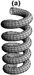
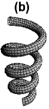
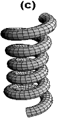
Figure 2: Helical solutions of the Kirchhoff equations using the Lancret’s Theorem. (a) circular helix solution valid for a rod with constant bending coefficient $B_{a}=1$ (47); (b) and (c) are generalized helices for inhomogeneous rod with bending coefficient given by Eqs. (48) and (49), respectively. The parameters, in scaled units, are $M_{3}=0.05$, and the total length of the rod is $L=130$. $k_{F}(0)=0.24$ for the helical solutions displayed in panels (a) and (b), and $k_{F}(0)=0.22$ for panel (c).

The tridimensional helical configurations displayed in Fig. 2 were obtained by integrating the Frenet-Serret equations (44-46) using the following initial conditions for the Frenet frame: ${\mathbf{t}}(s=0)=(0,\sin\alpha,\cos\alpha)$, ${\mathbf{n}}(s=0)=$ $(-1,0,0)$ and ${\mathbf{b}}(s=0)=$ $(0,-\cos\alpha,\sin\alpha)$, where $\alpha$ represents the angle between the tangent vector ${\mathbf{t}}$ and the helical axis. This choice ensures that the $z$-axis is parallel to the direction of the helical axis. The centerline of the helical rod is a space curve ${\mathbf{x}}(s)=(x(s),y(s),z(s))$ that is obtained by integration of the tangent vector ${\mathbf{t}}(s)$. We have placed the initial position of the rod at $x(0)=1/k_{1}(0)$, $y(0)=0$ and $z(0)=0$ (in scaled units), where $k_{1}(0)$ is the curvature of the projection of the helical centerline onto the plane perpendicular to the helical axis. It is possible to show [30] that

$$x(0)=\frac{1}{k_{1}(0)}=\frac{k_{F}(0)\,B^{2}(0)}{M_{3}^{2}+k_{F}^{2}(0)B^{2}(0)}\;.$$ (50)

$k_{F}(0)$ and $M_{3}$ are free parameters that have been chosen so that the helical solutions displayed in Fig. 2 have the same angle $\alpha$. The parameters $k_{F}(0)=0.24$ and $M_{3}=0.05$ give $x(0)\simeq 4$ for the helical solutions displayed in Figs. 2a and 2b, and the parameters $k_{F}(0)=0.22$ and $M_{3}=0.05$ give $x(0)\simeq 4.36$ for the helical solution displayed in the Fig. 2c.

5 Conclusions

The existence of circular (planar ring) and helical configurations for a rod with non-constant bending and twisting stiffnesses has been investigated within the framework of the Kirchhoff rod model. We are interested in finding analytical solutions, and since the static Kirchhoff equations consist of nine non-linear PDEs, we derived from them a set of differential equations (Eqs. (18–20)) for the curvature, $k_{F}$, and torsion, $\tau_{F}$, of the rod centerline, and then applied the geometric conditions to obtain circular and helical solutions.

We have shown that the planar ring ($k_{F}=$ Constant) is an equilibrium solution of the Kirchhoff equations for an inhomogeneous rod which possesses the bending stiffness, $B(s)$, satisfying Eq. (26), and $f_{3}(s)$ satisfying Eq. (30). The planar ring is the only planar solution for twisted rods ($M_{3}\neq 0$). Non-twisted rods ($M_{3}=0$) may present other types of planar solutions with $k_{F}(s)$ (non-constant) satisfying Eq. (28).

We also have shown that the circular helix is a solution of the static Kirchhoff equations only if the rod bending coefficient $B=$ Constant (see Eq. (43)). An inhomogeneous rod has $B\neq$ Constant, therefore it cannot have a circular helix as equilibrium solution. Nevertheless, it can exhibit generalized helical structures that satisfy the Lancret’s theorem, Eq. (32). In the Kirchhoff model, these generalized helical solutions can be obtained solving Eq. (35) for $\tau_{F}(s)$. Figure 2 displays three examples of helical structures that satisfy the static Kirchhoff equations.

May an intrinsically straight homogeneous elastic rod present other types of generalized helical equilibrium solutions ? A homogeneous rod has $C$ constant, implying $k_{3}=$ Constant (from Eq. (13)). It has been proved that $\xi^{\prime}=0$ for a helical solution of a homogeneous rod (see reference [35]), and Eq. (17) shows that the torsion $\tau_{F}=k_{3}=$ Constant. In order to satisfy the Lancret’s theorem (Eq. (32)), the curvature $k_{F}$ of this helical solution must also be constant. Since the helical structure whose curvature, $k_{F}$, and torsion, $\tau_{F}$, are constant, is a circular helix, the only type of helical solution for an intrinsically straight homogeneous rod is the circular helix.

Some motivations for this work are related to defects [36] and distortions [37] in biological molecules. Also, the stiffness of the DNA molecule has been proved to be sequence-dependent [3]. These defects, distortions and sequence-dependent elastic properties could be modeled as inhomogeneities along a continuous elastic rod.

Haijun and Zhong-can [34] have used the Goriely and Tabor stability analysis method [22, 23] to explain the onset of instability in the phenomenon of kink formation in small closed DNA molecules reported by Han et al [38, 39]. In the Han et al experiment [39], the DNA rings are immersed in a solution containing Zn²⁺ or Mg²⁺ ions. They found that DNA rings become kinked when the concentration of Zn²⁺ ions is above a critical value, with or without the presence of Mg²⁺ which alone did not produce the kinking phenomenon. Haijun and Zhong-can proposed that the binding of Zn²⁺ ions to DNA basepairs enhance the intrinsic curvature of the DNA destabilizing it. The Mg²⁺ ion, by binding to the phosphate backbone, did not produce intrinsic curvature in the DNA molecules. Nevertheless, Haijun and Zhong-can theory did not explain how the binding of Zn²⁺ ions lead to a variation of the curvature of the closed DNA. Also, the asymmetries and positions of the kinks in the DNA rings have not been explained.

Our approach can give a new insight to the phenomenon of kink formation of these closed DNAs. Due to the binding of the Zn²⁺ ion to a basepair, the bending stiffness of the DNA molecule should decrease locally, leading to a local increase of curvature. On the other hand, the binding of the Mg²⁺ ion to the phosphate backbone cannot change the stiffness of the molecule since the phosphate backbone is a very rigid structure. Our model supports this proposal since the equilibrium solutions represented by Eq. (31) show that the curvature is inversely proportional to the bending stiffness. Also Eq. (31) is only valid for a non-twisted rod which is the case of the DNA rings reported in Ref. [38, 39].

Haijun and Zhong-can have shown that closed DNA with curvature above a critical value never forms kinks in presence of Zn²⁺ or Mg²⁺ ions. It explains why Han et al [39] frequently observed kinks in closed DNAs of 168 basepairs (bps) long, while they rarely observed kinks in closed DNAs of 126-bps long, independent of the presence of Zn²⁺ ions in the solution containing the DNA rings. However, Haijun and Zhong-can approach cannot explain the approximate elliptical shapes of the 126-bps circles observed by Han et al [39]. Our results suggest that the non-circular shape of the 126-bps closed DNAs is a consequence of the binding of Zn²⁺ ions to the basepairs that decreases locally the stiffness of the DNA, thus increasing the curvature.

It has been proposed [40, 41, 42] that the kinking phenomenon is an important mechanism for wrapping DNA around nucleosomal proteins. In 1997, Luger et al [43] reported the X-ray crystalline structure of the nucleosomal protein, demonstrating that the DNA is not uniformly bent around nucleosome, but presents minimum and maximum curvatures at different positions. It is well known that the stiffness of DNA is sequence-dependent. Our results show that the variation of the bending stiffness of the DNA can give rise to these minimum and maximum curvatures.

Appendix A Appendix: The differential equations for the curvature and torsion

Here, we shall derive the Eqs. (18–20). Substitution of Eqs. (15–17) into Eqs. (8–13) gives:

$$f^{\prime}_{1}-f_{2}\,(\xi^{\prime}+\tau_{F})+f_{3}\,k_{F}\cos\xi=0\;,$$ (51)

$$f^{\prime}_{2}+f_{1}\,(\xi^{\prime}+\tau_{F})-f_{3}\,k_{F}\sin\xi=0\;,$$ (52)

$$f^{\prime}_{3}-f_{1}\,k_{F}\cos\xi+f_{2}\,k_{F}\sin\xi=0\;,$$ (53)

$$(B(s)\,k_{F}\sin\xi)^{\prime}+(C(s)-B(s))\,k_{F}\cos\xi\,(\xi^{\prime}+\tau_{F})-f_{2}=0\;,$$ (54)

$$(B(s)\,k_{F}\cos\xi)^{\prime}-(C(s)-B(s))\,k_{F}\sin\xi\,(\xi^{\prime}+\tau_{F})+f_{1}=0\;,$$ (55)

$$(C(s)\ (\xi^{\prime}+\tau_{F}))^{\prime}=0\;.$$ (56)

First, we extract $f_{1}$ and $f_{2}$ from Eqs. (55) and (54), respectively:

$$f_{1}=-(B(s)\,k_{F})^{\prime}\cos\xi+[M_{3}\,k_{F}-B(s)\,k_{F}\,\tau_{F}]\sin\xi\;,$$ (57)

$$f_{2}=(B(s)\,k_{F})^{\prime}\sin\xi+[M_{3}\,k_{F}-B(s)\,k_{F}\,\tau_{F}]\cos\xi\;,$$ (58)

where $M_{3}=C(s)\,(\xi^{\prime}+\tau_{F})$ is the torsional moment of the rod that is constant by Eq. (56). Differentiating $f_{1}$ and $f_{2}$ with respect to $s$, substituting in Eqs. (51) and (52), respectively, and using Eqs. (57) and (58), gives the following equations:

$$\begin{array}[]{ll}\left\{-(B(s)\,k_{F})^{\prime\prime}-\tau_{F}[M_{3}\,k_{F}-B(s)\,k_{F}\,\tau_{F}]+f_{3}\,k_{F}\right\}\,\cos\xi\,\,\,+\\ \left\{[M_{3}\,k_{F}-B(s)\,k_{F}\,\tau_{F}]^{\prime}-\tau_{F}(B(s)\,k_{F})^{\prime}\right\}\,\sin\xi=0\;,\end{array}$$ (59)

$$\begin{array}[]{ll}\left\{(B(s)\,k_{F})^{\prime\prime}+\tau_{F}[M_{3}\,k_{F}-B(s)\,k_{F}\,\tau_{F}]-f_{3}\,k_{F}\right\}\,\sin\xi\,\,\,+\\ \left\{[M_{3}\,k_{F}-B(s)\,k_{F}\,\tau_{F}]^{\prime}-\tau_{F}(B(s)\,k_{F})^{\prime}\right\}\,\cos\xi=0\;.\end{array}$$ (60)

Multiplying Eq. (59) (Eq. (60)) by $\sin\xi$ ($\cos\xi$) and then adding the resulting equations, we obtain the Eq. (18) for the curvature and torsion:

$$[M_{3}\,k_{F}-B\,k_{F}\,\tau_{F}]^{\prime}-(B\,k_{F})^{\prime}\tau_{F}=0\;.$$ (61)

Multiplying Eq. (59) (Eq. (60)) by $-\cos\xi$ ($+\sin\xi$) and then adding the resulting equations, we obtain the Eq. (19):

$$(B\,k_{F})^{\prime\prime}+k_{F}\,\tau_{F}(M_{3}-B\tau_{F})-f_{3}\,k_{F}=0\;.$$ (62)

Finally, the Eq. (20) is obtained by substituting Eqs. (57) and (58) in Eq. (53):

$$(B\,k_{F})^{\prime}+f_{3}^{\prime}=0\;.$$ (63)

References

- [1] E. E. Zajac, J. Appl. Mech. 29 (1962) 136.
- [2] J. Coyne, IEEE J. Ocean. Eng. 15 (1990) 72.
- [3] T. Schlick, Curr. Opin. Struct. Biol. 5 (1995) 245. W. K. Olson, Curr. Opin. Struct. Biol. 6 (1996) 242.
- [4] C. W. Wolgemuth, T. R. Powers, R. E. Goldstein, Phys. Rev. Lett. 84 (2000) 1623.
- [5] D. N. McIlroy, D. Zhang, Y. Kranov, M. Grant Norton, Appl. Phys. Lett. 79 (2001) 1540.
- [6] A. F. da Fonseca, D. S. Galvão, Phys. Rev. Lett. 92 (2004) 175502.
- [7] W. M. Huang, Mat. Sci. Eng. A 408 (2005) 136.
- [8] A. F. da Fonseca, C. P. Malta, D. S. Galvao, J. Appl. Phys. 99 (2006) 094310.
- [9] A. Mielke, P. Holmes, Arch. Rational Mech. Anal. 101 (1988) 319.
- [10] M. A. Davies, F. C. Moon, Chaos 3 (1993) 93.
- [11] G. Domokos, P. Holmes, Int. J. Non-Linear Mech. 28 (1993) 677.
- [12] A. F. da Fonseca, C. P. Malta, M. A. M. de Aguiar, Physica A 352 (2005) 547.
- [13] A. F. da Fonseca, M. A. M. de Aguiar, Physica D 181 (2003) 53.
- [14] A. F. Fonseca, M. A. M. de Aguiar, Phys. Rev. E 63 (2001) 016611.
- [15] A. Goriely, T. McMillen, Phys. Rev. Lett. 88 (2002) 244301.
- [16] A whip is a nonhomogenous thread with varying radius of cross section.
- [17] H. Kashimoto, A. Shiraishi, J. Sound and Vibration 178 (1994) 395.
- [18] J. Neuringer, I. Elishakoff, Proc. R. Soc. Lond. A 456 (2000), 2731.
- [19] G. Kirchhoff, J. Reine Anglew. Math. 56 (1859) 285.
- [20] E. H. Dill, Arch. Hist. Exact. Sci. 44 (1992) 2.
- [21] M. Nizette, A. Goriely, J. Math. Phys. 40 (1999) 2830.
- [22] A. Goriely, M. Tabor, Physica D 105 (1997) 20.
- [23] A. Goriely, M. Tabor, Nonlinear Dynamics 21 (2000) 101.
- [24] I. Tobias, D. Swigon, B.D. Coleman, Phys. Rev. E 61 (2000) 747; B.D. Coleman, D. Swigon, I. Tobias, Phys. Rev. E 61 (2000) 759.
- [25] A. Goriely, M. Tabor, Proc. R. Soc. London, A 453 (1997) 2583.
- [26] A. Goriely, P. Shipman, Phys. Rev. E 61 (2000) 4508.
- [27] A. Goriely, M. Nizette, M. Tabor, J. Nonlinear Sci. 11 (2001) 3.
- [28] N. Chouaieb, J. H. Maddocks, J. Elasticity 77 (2004) 221; N. Chouaïeb, PhD Thesis, École Polytechnique Fédérale de Lausanne, 2003.
- [29] M. P. do Carmo, Differential Geometry of Curves and Surfaces, Prentice Hall, Inc. Englewood Cliffs, New Jersey, 1976.
- [30] D. J. Struik, Lectures on Classical Differential Geometry, 2nd Edition, Addison-Wesley, Cambridge, 1961.
- [31] S. Neukirch, M. E. Henderson, J. Elasticity 68 (2002) 95.
- [32] The references in [20] can be seen for a complete derivation of the Kirchhoff equations.
- [33] J. Langer, D. A. Singer, SIAM Rev. 38 (1996) 605.
- [34] Zhou Haijun, Ou-Yang Zhong-can, J. Chem. Phys. 110 (1999) 1247.
- [35] T. McMillen, A. Goriely, J. Nonlin. Sci. 12 (2002) 241.
- [36] W. A. Kronert et al, J. Mol. Biol. 249 (1995) 111.
- [37] V. Geetha, Int. J. Biol. Macromol. 19 (1996) 81.
- [38] W. H. Han, S. M. Lindsay, M. Dlakic, R. E. Harrington, Nature (London) 386 (1997) 563.
- [39] W. Han, M. Dlakic, Y.-J. Zhu, S.M. Lindsay, R.E. Harrington, Proc. Natl. Acad. Sci. U.S.A. 94 (1997) 10565.
- [40] J. A. Schellman, Biopolymers 13 (1974) 217.
- [41] F. H. Crick and A. Klug, Nature (London) 255 (1975) 530.
- [42] H. M. Sobell, C. Tsai, S. G. Gilbert, S. C. Jain and T. D. Sahore, Proc. Natl. Acad. Sci. USA 73 (1976) 3068.
- [43] K. Luger, A. W. Mäder, R. K. Richmond, D. F. Sargent and T. J. Richmond, Nature (London) 389 (1997) 251.