Virtual volatility

Abstract

We introduce the concept of virtual volatility. This simple but new measure shows how to quantify the uncertainty in the forecast of the drift component of a random walk. The virtual volatility also is a useful tool in understanding the stochastic process for a given portfolio. In particular, and as an example, we were able to identify mean reversion effect in our portfolio. Finally, we briefly discuss the potential practical effect of the virtual volatility on an investor asset allocation strategy.

1 Introduction

Return on investment is a central concept for investors.  We here consider the simplest case of buying and holding a stock which, to make things easy, has no dividends or stock splits during the holding period. We assume a buy and hold strategy which ends at a horizon time $T$ later. In this paper, we are primarily interested in horizon times $T\,\$of the order of a year. [We do not treat the important issue of diversification and correlations between the returns of different stocks. To some extent, this can be treated by considering the entire portfolio in place of a single stock.]

The return can be defined as

$$R_{T,t}=\ln(S_{T+t}/S_{t})$$ (1)

where $S_{t}$ is the cost of the stock per share at time $t$ in the buy transaction, and $S_{T+t}$ is the amount to be realized per share at the time $T+t$ of the selling transaction. This is easy enough to calculate after the transactions are history. That result is called the historical return.

Some idea of what the return is expected to be when the decision is made to buy or not buy the stock is essential however.  The problem is to predict, ex ante, the stock price at a time in the future. It is universally accepted that there is a stochastic component to the changes in price. This leads inexorably to the idea that the best that can be hoped for is a prediction of the probability distribution  [PDF] of returns at time $T+t$, which we call $p_{t}(R|T)$.  It is fairly generally accepted that for most stocks the distribution is likely to be more or less bell-shaped, with a ‘center’ parameter and a ‘width’ parameter.  ‘Skewness’ and ‘fatness of tail’ parameters are also interesting but shall not concern us here.

We arrive at the conclusion, as many others have done, that for horizon times of a year, this distribution of returns can be taken to be normal, [log-normal for the stock], at least as a reasonable starting point. This means that the main two parameters are the width and the center parameter. The latter is generally taken to be the expected or mean return, which we define as

$$\mu_{T}=E_{t}(R_{T})=\int dR~{}R\,p_{t}(R|T)$$ (2)

The width $\sigma_{T}$ is usually determined from $v_{T}=\sigma_{T}^{2}$ , the variance of the distribution

$$v_{T}=E_{t}\left(\left[R_{T}-\mu_{T}\right]^{2}\right)$$ (3)

[An equivalent and perhaps more popular definition of the ‘mean return’ is $\tilde{\mu}_{T}$, defined as $\tilde{\mu}_{T}=\ln\left(E\left(S_{T+t}/S_{t}\right)\right).$ If the PDF is lognormal, $\tilde{\mu}_{T}=\mu_{T}+\frac{1}{2}v_{T}.]$

The dependence of the PDF on $t$ emphasizes that the distribution is that predicted at time $t.$ This PDF is exceptionally important because it is the one that is acted on by the investor. It is conditional on past history, including the price $S_{t}$ as well as all other information and theory that the investor is able to bring to bear. Thus, in a sense there is a different PDF for every investor. Of course, it’s probably true that only a small fraction of investors think in terms of PDF’s. What follows is in the nature of advice to those few investors on how to improve systematically their PDF’s.

The expected return is also called the drift. The latter terminology comes from the random walk model discussed further below. The parameter $\sigma_{T}$ is one among several distinct definitions of the volatility.   The volatility is almost always, in spite of cogent criticisms, taken to be practically synonymous with the concept of risk. It is obviously a sort of inverse predictability, the larger the volatility, the less the horizon price is predictable. The whole point of this paper is to discuss this volatility and its relationship to the concept of drift.

This class of distributions of stock prices in the future must be sharply distinguished between somewhat similar distributions in common use. One example is the unconditional distribution of Lo and Wang, [1],LW, which ‘fixes’ the parameters, (including $\mu$ and $\sigma)$ at their ‘true’ values. [Quotes are as in LW]. Another is the ‘risk neutral world’ PDF used in option pricing theory, which is usually stated to be the distribution of the price of the underlying stock at the future time $t+T,$ with the drift parameter $\tilde{\mu}_{T}$ replaced by the risk-free return $rT.$ We think, that there is an explicit formula for what to use as the option pricing volatility parameter giving a result $\sigma_{BS}$ related to the Black-Sholes theory [2, 3, 4]. Closely related to this is the risk free world distribution in which the volatility parameter is the ‘implied’ volatility, $\sigma_{I}$ extracted from empirical option prices [4]. The implied volatility in effect incorporates a number of corrections to that of Black-Sholes. Although these volatilities are correct for option pricing purposes, we show that neither of these volatilities is correctly used as the standard deviation of $p_{t}(R|T).$

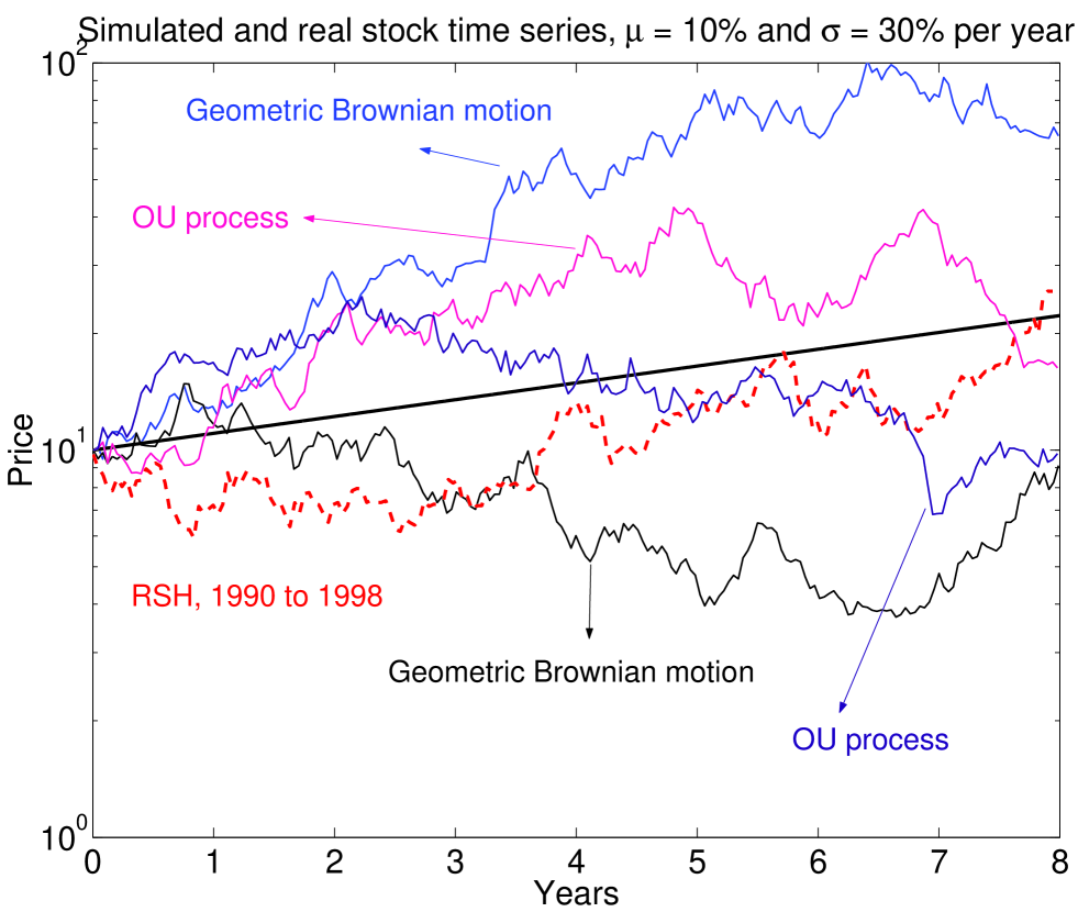
Suppose we have the daily price history of a single stock over a year. Assume for the sake of argument that this history is generated by a Monte Carlo program with constant parameters, whose numerical values are in the range expected for stocks, but we don’t know the parameters (Fig. 1). The exercise is to estimate the parameters from the data. We will argue that we can determine the width parameter $\sigma_{BS}$ fairly well from the data of a single year.

From a single year’s data, the best we can do to estimate the expected return is $\mu_{T}\approx R_{T}\pm\sigma_{BS}$, which will get the sign wrong fairly often (Fig. 1). It is certainly known that it is impossible to measure the historical mean drift very well. Decades of data would be needed, even on the dubious assumption that the drift and other parameters are constant over those decades[5]. Predicting the expected return parameter is even harder. It is nevertheless routine to act as if the drift parameter is ‘fixed’ at its ‘true’ value.

To obtain the parameters of the yearly distribution, the Monte Carlo for a year could be run many times. This is something that cannot be done for an actual security. If the program were for a standard random walk, as is assumed for simplicity by Black-Sholes and the efficient market hypothesis, that would determine $\mu_{T}$ and it would be found that the yearly width is $\sigma_{BS.}$ If the program were for a mean reverting Ornstein-Uhlenbeck [OU] process the result would be a width $\sigma_{OU}<\sigma_{BS},$ and the result would depend on another parameter $\gamma,$ the rate of reversion to the mean. We estimate crudely below that $\gamma^{-1}$ is of the order of 1 year for actual stocks. Other stochastic models are by no means ruled out empirically.

Figure 1: Stock price time series for simulated and one real stock (RSH, Radio Shack) with similar mean return and volatility of $\sigma=0.3$ and $\mu=0.1$ per year. The smallest time step for the simulation is $1$ day. The solid black line represent the mean drift of $0.1$ per year. Note that it is not possible to extract the correct mean return by simply looking at one t simulated time series. Therefore it is questionable to assume that RSH comes from a random process presenting $10\%$ mean return. All we can say is that RSH had a realized return of $10\%$ for the period in question. It is also difficult to distinguish between different stock process. For comparison we present $2$ simulated processes. One is the traditional geometrical Brownian motion, the second is an OU process with a target price of $15$ dollars after $1$ year. Both are similar if we look at few time series.

The main, albeit quite intuitive, result of this paper is as follows: Clearly, since one doesn’t know the drift very well, one should make some sort of average over the reasonable predictions of that parameter. This leads to a systematic result: the volatility of a predicted stock price, as defined by Eq.(3) is greater than the volatility of the unconditional distribution, and also greater than the volatilities $\sigma_{BS}$ or $\sigma_{I}.$ We call this enhanced volatility $\sigma_{T},$ as above, and we estimate empirically, using $304$ companies which are part of the S&P500 , that $\sigma_{T}\approx\left(1.26-1.34\right)\sigma_{BS}.$ We call this 26-34% enhancement, the virtual volatility, which comes, not because of a stochastic process, but because of our inability to predict or even measure accurately, the mean return. In other words, this is not the standard deviation of any given process, but rather that of an ensemble of processes, an ensemble which is virtual because it exists only in our heads.

Finally we point out a remarkable and often overlooked consequence to investors of the existence of the virtual volatility.

2 Theoretical and Empirical Distributions of Returns

In the stock market, where every day billions of dollars generate gigabytes of data, one might think that reasonable empirical estimates of the distribution of such a fundamental quantity as the return would be commonplace. This is true, but only for short horizon times. For example, suppose $T$ = 1 hour. It is then plausibly assumed that, except for stochastic processes, the return during each hour is the same. So, one could let $t$ in Eq.(1) run over each hour for a couple of years to obtain a large number of exemplars. The hourly mean return is in one sense known very well. Namely, it is much smaller than the hourly volatility. However, it not known well enough to use it to estimate very well the annual mean return, even on the assumption that the hourly return is constant.

Of course, one should not really include every hour, just every trading hour. Or perhaps the returns during the final hour of each trading day, or maybe the last hour on Fridays or before holidays could be examined. These are conditional distributions, all hourly, which are known to be significantly different from one another. It is for some purposes quite acceptable to average over all the constraints (except for not including nontrading hours).

It is known that for short horizons, up to a week, say, that the shape of the empirical returns depends significantly on $T.$ At minutes, there are power law tails and significant correlation between successive minutes [6, 7, 8]. At hours or days, the main part of the return is approximately exponential, with little apparent correlation between one day and the next. At still longer times the return distribution evolves in the direction of normality [6, 7, 8]. However, for these longer times, quarters, years, decades, one should not in general assume that all the underlying parameters are constant for a given stock for a sufficient length of time that an empirical distribution obtained from the time series of a single stock is well defined. Certainly, for horizons much longer than a year, the supposition that the parameters are constant is hard to justify.

The reason for this trend to normality is of course the Central Limit Theorem. There are many small reasons for the changes in price of a stock. These reasons have fairly short time scale parameters. In the course of a year, the fluctuations with short time characteristics get averaged out.

To make progress, one needs to invoke some theory. We assume that the stock follows a generalized random walk with finite time increment $\Delta t$. It is usual in academic economic theory to take $\Delta t$ as an infinitesimal, in order to connect to the beautiful theory of stochastic differential equations, but, as we have just seen, there is much going on at short times that only indirectly affects the yearly behavior. So we think of $\Delta t$ as being some interval like a day, short compared with $T,$ but long enough to minimize intraday effects.

Let $s_{t}=\approx\left(S_{t+\Delta t}-S_{t}\right)/S_{t}=\Delta S_{t}/S_{t}.$ Then we assume something like Brownian motion, or a random walk,

$$s_{t}=\mu_{t}\Delta t+\sigma_{t}\Delta t^{1/2}W_{t}.$$ (4)

Here $W_{t}$ is a random number of mean zero and unit variance. The daily drift $\mu_{t}\Delta t$ is small, and for our purposes nonstochastic, but it can be a function of time and past history. The daily standard deviation $\sigma_{t}\Delta t^{1/2}$ can be constant, time dependent, or even mean reverting stochastic with correlations [8], but we assume that maximum correlation times for the daily volatility are such that most of the effects of volatility fluctuations are averaged out over times of order a year. We assume that $\left(\mu_{t}\Delta t\right)^{2}<<\sigma_{t}^{2}\Delta t.$  [This is based on the estimate that the drift for a year is typically in the range 10-20%, while the volatility for a year is 20-40%.  Let $\Delta t$ be about $1/252$ years. Then $\left[.15/252\right]^{2}=4\times 10^{-7}<<4\times 10^{-4}=.3^{2}/252.$] This is a very fundamental inequality. It says that at short times, $\Delta t\approx$ a day, the drift is so small that for most purposes it can be neglected.

The usual Black-Sholes theory of option pricing takes $\mu_{t}$ and $\sigma_{t}$ as constants. This is unnecessary and we can consider them to be time dependent [1]. We adopt units of time such that $\Delta t=1$ and then $T$ is large, e. g. one year $\approx$ 252 trading days. Theory shows that the distribution of $R_{T,0}=\Sigma_{t=0}^{T-1}s_{t}$ is then normal with drift parameter $\Sigma\mu_{t}=T\bar{\mu}$ and width parameter $\sqrt{\Sigma\sigma_{t}^{2}}.$ The Black-Sholes price is based on hedging. Then there is a natural ‘short’ time which disappears in the continuous version of the theory. This fundamental short time is the interval between rehedgings. If this time is too short, transaction costs become excessive. If it is too long, the expansion given below breaks down. Although it is in reality more complicated, assume for simplicity that the time between rehedging is $\Delta t=1$ day. The dealer sells an option and maintains a hedge. Let the number of hedge shares owned between time $t$, $t+1,$ be $\phi_{t}.$ Assume the risk free rate is zero, as it is known how to restore it to the formulas by a trick at the end. Invoking the usual no-arbitrage condition, the change in value of the hedge of the dealer from time $t$ to time $t+1,$ but just before rehedging, is equal to the change in his obligation to the buyer, i.e. to the change of the fair value or price $C(S_{t,}t)$ of the option. Thus, using a Taylor expansion to calculate the change of price we have

$$\Delta S_{t}\phi_{t}=C(S_{t+1},t+1)-C(S_{t},t)\\ \approx\Delta S_{t}\frac{\partial C}{\partial S_{t}}+\frac{1}{2}\frac{\Delta S_{t}^{2}}{S_{t}^{2}}S_{t}^{2}\frac{\partial^{2}C}{\partial S_{t}^{2}}+\frac{\partial C}{\partial t}+...$$

Black-Sholes make the ‘delta’ hedge $\phi_{t}=\partial C/\partial S_{t},$ and choose the option price $C(S,t)$ as solution of the equation $\partial C/\partial t=-\frac{1}{2T}\sigma_{BS}^{2}S^{2}\partial^{2}C/\partial S^{2},$ where obviously the ‘constant’ $\sigma_{BS}^{2}/T$ should be given by

$$\sigma_{BS}^{2}=\Sigma_{t}\Delta S_{t}^{2}/S_{t}^{2}=\Sigma(\mu_{t}+\sigma_{t}W_{t})^{2}\approx\Sigma\sigma_{t}^{2}=T\overline{\sigma_{t}^{2}}$$ (5)

if $T$ is large, and $\mu_{t}$ is small in the sense above. Note that for large $T,$ $\sigma_{BS}^{2}\propto T.$ Also, the ‘miracle’ has happened, the option price does not depend on the drift parameter.

Furthermore, the future Black-Sholes volatility, (for $T\approx one$ $~{}year),$ is rather well predicted by the historical data. The Black-Sholes volatility (divided by the horizon time) is and should be, an average ‘daily’ volatility, daily because of the ‘daily’ rehedging, and not necessarily the width of the distribution at time $T,$ predicted by Eq. (4). Therefore, one has rather good statistics, since there are many days until time $T+t$ is reached. However, if $\mu_{t}$ is some ‘known’ simple function of $t,$ which maintains the smallness constraints, Eq.(4) does predict a width $\sigma_{BS}.$

Let us next suppose that $\mu_{t}$ has a mean reversion property. Namely, let us suppose that $\mu_{t}$ ‘points’ to some future price goal $S_{G}(t+1/\gamma)$, at a time $1/\gamma$ in the future. It points in the sense that $S_{t}e^{\mu_{t}/\gamma}=S_{G}(t+1/\gamma)$ or $\mu_{t}=\gamma(\ln S_{G}-\ln S_{t}),$ Suppose that $S_{G}(t)=S_{G}e^{\mu t}.$ Then, Eq.(4) becomes

$$s_{t}=-\gamma(\ln S_{t}-\ln S_{G}-\mu t)\Delta t+\mu+\sigma_{t}\sqrt{\Delta t}W_{t}$$ (6)

which is a simple trending Ornstein-Uhlenbeck process. It has three drift related parameters, $\mu,$ $S_{G},$ and $\gamma.$ Both $S_{G}$ and $\mu$ are difficult to extract from the data on a single stock. Let

$$\,q_{t}=\ln S_{t}/S_{G}-\mu t.$$ (7)

Note that one expects $\overline{\left|q_{t}\right|}\approx\sigma_{t}/\sqrt{\gamma}$ so that for this process $\mu_{t}^{2}\approx\gamma\sigma_{t}^{2}<<\sigma_{t}^{2}$ if $\gamma\approx 1/250$, i.e. $\gamma$ is an inverse year. Thus, the Black-Sholes option price is not changed if the underlying process is mean reverting rather than a random walk, and is again determined by the average daily variance [1, 9].

The volatility of the future distribution predicted by the OU process has a different value, however. It is given by $\sigma_{OU}^{2}=\sigma_{BS}^{2}\left(1-e^{-\gamma T}\right)/\gamma T.$ There is also a negative correlation between successive returns, $E_{OU}(\left(R_{T,t}-\mu T\right)\left(R_{T,t-T}-\mu T\right))=-\frac{1}{2}\sigma_{OU}^{2}\left(1-e^{-\gamma T}\right)$ [1]. [These results are easily obtained by use of an explicit solution for $q_{t}=\Sigma_{s=-\infty}^{t}\sigma_{s}e^{-\gamma\left(t-s\right)}W_{s},$ which can be approximated as a stochastic integral. Because we don’t know $S_{G},$ we don’t know the value of $q_{0}$ at time $t=0$ even if we know the price $S_{0}$ at that time. Setting the lower limit in the sum far into the past makes $q_{0}$ a stochastic quantity and supplies a sort of average over $S_{G}$. The results are different if $S_{G}$ and $S_{0}$ are known.]

Another model with some plausibility is one in which the drift is constant for a while, probably of order a year, then in a short time of a month or two jumps to a new constant. This process would have to be mean-reverting also. Since it requires even more parameters and is not well worked out, we do not discuss it further.

3 Averaging over predicted mean returns

Our idea is to assume an underlying random walk or trending OU process, where the chief unknown parameter is the expected return $\mu_{t}$. If we knew this parameter, the PDF would be log normal with the width dependent on the process. Our recommendation to the subset of investors who try to estimate a stock’s future PDF, is that they average somehow over reasonable predictions of the expected return, which will result in a distribution that is wider than the underlying widths $\sigma_{BS},$or $\sigma_{OU.}$

There are many schemes utilized to predict the future course of stocks. There are at least three general methodologies. Value investors believe that such underlying factors as earnings, book value, cash flow, can be predicted and can be theoretically converted into a target price for the stock. Most research and commercial forecasting schemes like this are based on factor betting in the spirit of Fama and French [10, 11, 13, 12]. These schemes tend to predict target prices, which are related to the underlying ‘intrinsic value’ of the stock.

Another methodology is that of technical investing. Its proponents believe that various shapes of stock price history graphs give buy or sell signals. It is difficult to turn this into a prediction of the drift parameter.

One well documented version of technical investing is trend following or momentum investing [13, 14]. In that case it is assumed that what happened to the stock in the recent past is likely to continue for a while.

A third technique tries to take advantage of mean reversion. For example, one looks over a cross section of stocks and invests in those for which the recent returns have been unusually low. A value version is that one chooses stocks whose book to price ratio, say, is unusually high, in the expectation that the price will rise to bring the ratio down to more normal values [16].

It is apparent that not many of these techniques actually attempt to predict the expected return. In any case, it is not easy to extract such predictions from the published reports of analysts. The exception is momentum investing which assumes the actual return of the recent past can be used to predict the future [13, 14].

Figure 2: Empirical PDF for $304$ names from the S&P500 where the correlation between names is removed. Two random years are chosen for each name. Different random choices result in slightly different PDFs. The solid black line represents the best fit gaussian. The mean is approximately zero and the standard deviation is $1.30\pm 0.04$. We estimate the virtual volatility to be of the order of $26\%$ to $34\%$.

We still face the fundamental difficulty, stressed above, that for a given name, it is not possible to have enough exemplars of year-long price histories to determine the parameters. We must therefore go to a cross-sectional approach. Assume that we can choose a large number of similar names, which for the present purpose differ only by their mean drift and volatility[7]. If they are mean reverting, we assume their mean reversion parameters $\gamma$ are similar.

To compare one name with another, we normalize the returns. A natural first guess is the $t$- or Student statistic,

$$R_{T,Stud}=\frac{R_{T,t}-\bar{\mu}T}{\sigma_{BS,T,t}}$$ (8)

where $R_{T,t}=ln(S_{T+t}/S_{t})$ is the $T$ horizon return, the volatility is that measured over the period $t,t+T,$ and $\bar{\mu}$ is the ‘known’ average drift parameter. If the returns are normal, the distribution of the statistic of Eq.(8) will be a Student distribution with $T$ degrees of freedom. For large $T,$ this is nearly a normal distribution with zero mean and unit width.

However, we want to make a prediction based on history to time $t,$ so we replace the volatility in the denominator by the historical volatility. [Other approximations for $\sigma_{BS}$ work well also.]

Most importantly, we replace $\bar{\mu}T$ by an estimate which has a distribution. Namely we replace $\bar{\mu}T$ by the guess of the momentum investor, $\bar{\mu}T\rightarrow R_{T,t-T}=ln(S_{t}/S_{t-T})$. The result is a statistic which in effect averages the predictions of the drift as a momentum investor would do,

$$R_{T,norm}^{n}=\frac{R_{T,t}^{n}-R_{T,t-T}^{n}}{\sigma_{BS}^{n},_{t-T}}.$$ (9)

We add a label $n$ giving the name of the stock. Our interpretation of this statistic is that its width estimates the enhancement factor above the empirically known $\sigma_{BS}^{n}$ for the group of stocks due to the virtual volatility effect.

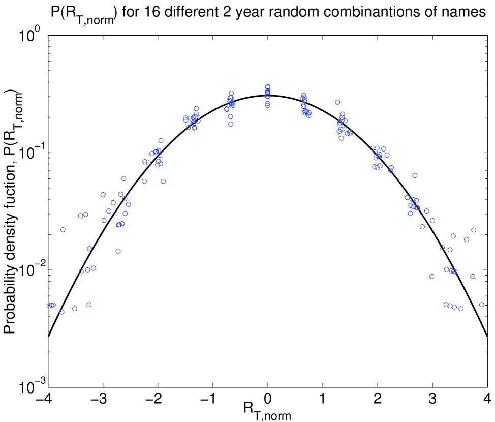
To illustrate this empirically, we take sixteen years of daily data ending Jan. 2006 of a $304$ stock subset of the S&P500. The subset was of stocks present in the S&P over the chosen time-span. [We have tried other time periods and other subsets with very similar results,including data that spans from Oct. 1993 to Oct. 2002.] The data was downloaded from Yahoo [15]. We deliberately wanted to have rather similar stocks, in this case rather large and actively traded companies, so that a cross sectional analysis has meaning.

One possible problem with the set of stocks we chose is that there is known to be considerable temporal correlation between stock price changes. Since studying the effects of correlation between names is not our interest here, we chose, for each name, three two year periods, at random, from the data. In other words, we took $T=252$ in Eq.(9) and $t$ was chosen at random in the interval Jan. 1990-Jan. 2006. This gives a sample of size $2430$ from which to estimate the distribution.

The distribution is normal with essentially zero mean and a width (standard deviation) about $1.26-1.34$ (Fig. 2). The normality of this distribution is consistent with the argument that year-in-the-future stock price distributions are lognormal. The zero mean is evidence that yearly past returns are unbiased predictors of yearly future returns. The width, 1.26-1.34, says that the volatility $\sigma_{T}$ of a given stock, a year in the future, is, on average, 26% - 34% greater than the empirical historical volatility for that stock. The reason for this increase in width or decrease in predictability is that we don’t know the ‘true’ drift parameter, but have effectively averaged it as a momentum investor would.

4 Mean Reversion

This result is the main result of this paper. However, the statistic defined by Eq.(9) has some nice features, even without the virtual volatility interpretation. This is especially true when $T$ is large enough that fluctuations in the empirically obtained denominator can be ignored or taken into account as a perturbation. One virtue, in contrast to the standard regression techniques used to study mean reversion, is that the double difference structure of the numerator of the statistic Eq.(8) is independent of drift parameters, known or unknown, if they are constant.

Let us assume first, that the $2430$ samples are generated by a random walk of Eq.(4) with constant drift parameters $\mu^{n}$, i. e. constant over two years for each choice of name and time interval. In each exemplar we may add and subtract the correct (even though unknown) $\mu^{n,t}$ in the numerator to find that such a random walk statistic theoretically has mean zero and variance two. In other words, a standard ensemble of random walks, but with unknown drift parameters, leads to a virtual volatility enhancement of $\sqrt{2}-1\approx 42\%.$ [Because of small fluctuations in the denominator, it is actually slightly larger.]

Real stocks are therefore more predictable than the random walk with constant but unknown parameters itself. The reason is that real stocks are mean reverting [16, 17, 18]. Some argue that mean reversion contradicts the idea of market efficiency, therefore it is sometime termed an anomaly [16].

Suppose we assume that the stocks of Eq.(9) are mean reverting with the simple Ornstein-Uhlenbeck trending process. We take the reversion rate $\gamma$ constant over all time and all names. We also assume constant but unknown drift $\mu^{n}$ and fixed price target $S_{G}^{n}$ for each two year interval and name. The numerator of Eq.(9) can be expressed in terms of the normalized parameter $q_{t},$ Eq.(7), without needing to know the drift and target price. The result is:

$$var(R_{T,norm})=\left[\frac{(1-e^{-\gamma T})}{\gamma T}\right]\left[2+\left(1-e^{-\gamma T}\right)\right]$$ (10)

The first square bracket is the ratio of the Ornstein-Uhlenbeck variance of $R_{t\pm T}^{n}$ to the Black-Sholes volatility-squared of the same quantity. The parenthesis in the second square bracket comes from the negative correlation between history year and predicted year, as is characteristic of mean reversion.

From the numerical result for actual S&P stocks, we can conclude that an average $\gamma^{-1}$ is about 1.1 - 1.3 years for $T=1$ year, that is, the target price is a little above 1 year in the future. Assuming the same OU process applied to Fama and French results[17], we arrive at $1.9$ to $3.1$ years for small cap stocks and $4.3$ to $7.2$ years for large cap. Conversely our results indicate a correlation of one year returns of -0.32 (Fama and French find an insignificant correlation for one year returns). Our results are not in agreement with Fama and French, however we do not try to compare both. We have used different samples, different time periods and moreover we have assumed a very simple mean reversion model. We are only drawing the attention to the order of magnitude agreement we have achieved with a very crude model. If one takes seriously the OU model and formula 10, then the virtual volatility effect is enhanced, namely the actual width $\sigma_{T}\approx 1.5\sigma_{OU},$ for $T=1$ year.

However, real stocks are not so simple. Consider the empirical distribution of Eq.(9) for different values of $T.$ The results are given in Table 1.

Table 1: 1. The empirical estimate of the ratio of standard deviation of normalized log returns to the Black Sholes volatility, as a function of time horizon. 2. The rate of reversion to the mean calculated from the empirical estimate on the assumption that the stocks follow a simple trending OU process.

T(quarters)	1/3	1	2	3	4	5	6	7	8
$\sigma_{T}/\sigma_{BS}$	1.49	1.37	1.32	1.26	1.33	1.35	1.37	1.46	1.49
$\gamma^{-1}(years)$	**	7.7	2.4	1.15	1.3	1.2	1.3	**	**

The notation ** means that the simple OU process cannot give the result. Indeed, we can conclude that although the stocks are mean reverting, there is considerably more structure than found in the simplest OU process.

Since mean reversion is not the main subject of this paper, we confine ourselves to a simple, qualitative explanation of the table as follows. There is more than one time scale of stock price temporal correlation. In addition to the negative correlation at longer time [16, 17], there is a shorter time positive correlation at horizons of order week-month [6, 16, 18].

At still longer horizons, we suggest that the approximation that the drift $\mu_{t}$ is constant breaks down. If the drift is different for $R_{t+T}$ and $R_{T-t},$ there is a positive addition to the variance. Thus, $\dot{\sigma}_{T}/\sigma_{BS}$ has a minimum. In fact, for horizons of 7 and 8 quarters, the mean of $R_{T,norm}$ becomes distinctly negative. That means that the mean drift at the earlier time is on average greater than the mean drift at the later time. In other words, the returns earlier in the period were greater than the returns later in the period. Certainly for the market as a whole, during this period prices first went up during the ’90’s and turned over at about year 2000.

5 Investment consequences of the virtual volatility

We have just recounted arguments that the expected return parameter for a given stock or portfolio is not known very well and its value is not agreed on by market participants. We do not discuss the consequences of this for such concepts as the ‘efficient frontier’ of modern portfolio theory [MPT] [3, 19, 20, 21].

We argued that one way of thinking about this lack of knowledge and agreement on the expected return is that the PDF of future price distributions is wider than usually assumed, something like 1.3$\sigma_{BS}$. What are some of the consequences for investors? Since volatility is equated to risk in typical textbook finance, we see that stocks are risker by 30% than we thought they were. A favorite single number that tries to summarize how well a portfolio is going to perform, in the risk-return sense, is the ex ante Sharpe ratio, $Sr=\left(\mu_{T}-rT\right)/\sigma_{T}$. This number tries to balance the risk, defined as the volatility, with the return in excess of the risk free return. Obviously, it is reduced by 30% or so as compared with the ratio using the volatility $\sigma_{BS}.$ Going a bit beyond this is MPT, which uses of the utility functional $U(I_{0})=I_{0}(\mu_{T}-rT)-\frac{1}{2}AI_{0}^{2}\sigma_{T}^{2}.$ Here $A$ is the investor’s risk aversion parameter. Minimizing $U$ with respect to the investment amount, $I_{0},$ gives $I_{0}=\left(\mu_{T}-rT\right)/A\sigma_{T}^{2}$ which means that an investor using this MPT utility, would invest a factor 1.7 less because of the virtual volatility effect. The utility itself is changed to $U=\frac{1}{2A}Sr^{2}$, so the utility of the investment is reduced by the same rather significant factor.

It must be admitted that very few investors, (probably including Sharpe) know their personal value of the risk aversion parameter $A,$ so, all that needs to be done is to have everyone decrease their $A$ by a factor 1.7, in other words, become less risk averse than they had thought, and nothing would change. Thus, even though the previous calculation (without the virtual volatility effect) is in several textbooks, it is doubtful that it has much effect on live investors.

Nevertheless, it is clear and in agreement with intuition and standard lore, that additional uncertainty makes an investment less attractive.

There are, however, other ways of investing in stocks or indices than just buying them. One of the simplest is investing in calls on the underlying stock. In this paper we confine ourselves to pointing out the following. The expected excess gain, as predicted at the time of making the investment, for the strategy of buying a call at price $C_{K}$ and holding it until expiration at a time $T+t$ in the future, is given by

$$E_{t}[G]=I_{0}e^{rT}\left(\frac{E_{t}\left(\left(S_{T+t}-K\right)^{+}\right)}{C_{K}e^{rT}}-1\right)$$ (11)

Here $I_{0}$ is the amount invested, $S_{T+t}$ is the price of the underlying at expiration, and $K$ is the strike price. The expectation

$$E\left[\left(S_{Tt}-K\right)^{+}\right]=\int_{K}^{\infty}dS(S-K)p_{t}(S,\tilde{\mu}_{T},\sigma_{T})$$ (12)

where $p_{t}(S_{T+t},\tilde{\mu}_{T},\sigma_{T})$ is the ex-ante, predicted, log-normal distribution of final stock price that we have just discussed. The Black-Sholes call price [2, 4], (approximately $C_{K}),$ is given by the same formula, Eq. (12) with $p$ replaced by the risk neutral world distribution, $p(S_{T+t},rT,\sigma_{BS}).$ The actual call price is subject to various small corrections that are summarized by the replacement of $\sigma_{BS}$ by the implied volatility $\sigma_{I}.$ Thus $E(G)$ vanishes if $\tilde{\mu}_{T}=rT$ and $\sigma_{T}=\sigma_{I}.$[Note that Eq.(11) for $K=0$ gives the gain from buying the underlying when $C_{K=0}$ is the price of the stock, $S_{t}$.]

The expected gain is an increasing function of three parameters. The first, obviously, is the drift parameter $\tilde{\mu}_{T}.$ The second is the strike price $K.$ Both the numerator and denominator in Eq.(11) decrease with increasing $K,$ but the denominator decreases faster. [For options very much out of the money, $C_{K}$ is so small as predicted by Black-Sholes that the buy-sell option price spread starts to dominate.] The result is that somewhat out-of-the-money calls on stocks with projected good returns have considerably higher expected return than does the underlying itself, even if the volatility $\sigma_{T}$ is mistakenly kept at $\sigma_{I}$.

The third parameter is the virtual volatility $\sigma_{T}.$ As $\sigma_{T}$ increases, the expected return increases. The expected final call value of Eq.(12) increases, the more so for out of the money calls. The cost $C_{K}$ is independent of predictions of the future return. The wider virtual tails of $p(S_{T},\tilde{\mu}_{T},\sigma_{T})$ on the up side increase the return, while the losses coming from low side tails are limited to the cost of the call. The virtual volatility effect thus increases the expected return on call buying, without much increasing the prospect of losses. Similarly, if the actual distribution has fatter tails than the log-normal that we have assumed, it also raises the expected return without increasing much the prospect of losses. In fact, for out-of-the-money calls, there is a significant expected gain even if the return $\tilde{\mu}_{T}$ vanishes.

There is some empirical evidence which tends to support these ideas [22, 23]. That work of course has nothing to do with prediction. It did however find that the historical mean returns on certain rather short term ($\approx$ one month) calls was impressively high, the more so for out of the money calls.

A complete analysis requires a discussion of risk or utility in call-buying, a situation for which the ‘risk = volatility=standard deviation’ formulation of traditional MPT is far from adequate [24, 25]. We defer this discussion to a future publication. However, for those investors who are mainly averse to losing too much money, [as opposed to being averse to both upside and downside uncertainty equally,] it is quite clear that the virtual volatility effect as applied to calls increases the desirability of call buying, contrary to the outcome when purchase of the underlying is contemplated.

In other words, this is a case where certain rational investors can and should regard uncertainty and inability to predict correctly as GOOD!

We thank V. M. Yakovenko for several suggestions. We thank J-P. Bouchaud for pointing out Ref. [16].

References

- [1] A. W. Lo and J. Wang, Implementing option pricing models when asset returns are predictable. The Journal of Finance, 50, 87 (1995).
- [2] F. Black and M. Scholes, The pricing of options and corporate liabilities. Journal of Political Economy, 81, 637 (1973).
- [3] Z. Bodie, A. Kane and A. J. Marcus,Investments (McGraw-Hill, New York, 2002).
- [4] T. Bjork, Arbitrage theory in continuous time (Oxford University Press, New York, 1998).
- [5] F. Black, Estimating espected return. Financial Analysis Journal, Jan-Feb, 168 (1995).
- [6] J.Y. Campbell, Andrew W. Lo and A. C. MacKinley, The econometrics of financial markets (Princeton University Press, Princeton, 1997).
- [7] P. Gopikrishnan, V. Plerou, L. A. N. Amaral, M. Meyer, and H. E. Stanley, Scaling of the distribution of price fluctuations of individual companies. Phys. Rev. E 60, 6519 (1999).
- [8] A.C. Silva, R. E. Prange and V. M. Yakovenko, Exponential distribution of financial returns at mesoscopic time lags: a new stylized fact. Physica A, 344 227 (2004).
- [9] B. Grundy, Option prices and the underlying asset’s return distribution. The Journal of Finance, 46, 1045 (1991).
- [10] E. F. Fama and K. R. French, The cross-section of expected stock returns. The Journal of Finance, 47, 427 (1992).
- [11] J. L. Davis, E. F. Fama and K. R. French, Characteristics, Covariances, and Average Returns: 1929 to 1997. The Journal of Finance, 55, 389 (2000).
- [12] http://www.barra.com/products/model.aspx
- [13] M. Cooper, R. C. Gutierrez,Jr. and B. Marcum, On the predictability of stock returns in real time. The Journal of Business, 78, 460 (2005).
- [14] N. Jagadeesh and S. Titman, Returns to Buying Winners and Selling Losers: Implications for Stock Market Efficiency. The Journal of Finance, 48, 65 (1993).
- [15] http://biz.yahoo.com/opt/
- [16] W. F. M. De Bondt and R. H. Thaler, Anomalies: A mean-reverting walk down wall street. The Journal of Economic Perspectives, 3 189 (1989).
- [17] E. F. Fama and K. R. French, Permanent and temporay components of stock prices. The Journal of Political Economy, 96, 246 (1988).
- [18] A. W. Lo and A. C. MacKinlay, Stock Market prices do not follow random walks: evidence from a simple specification test. The Review of Financial Studies, 1, 41 (1988).
- [19] H. M. Markowitz, Portfolio selection. J. Finance 7,77 (1952).
- [20] H. Levy and H. M. Markowitz, Aproximating expected utility by a function of mean and variance. American Economic Review, 69 308 (1979).
- [21] C. Huang and R. H. Litzenberger, Foundations for financial economics (Prentice Hall, New Jersey, 1988).
- [22] J.D. Coval and T. Shumway, Expected option returns. The Journal of Finance 61, 983 (2001).
- [23] R. J. Rendleman Jr, Optimal long-run option investment strategies. Financial Management 10, 61 (1981).
- [24] P. Carr and D. B. Madan, Optimal positioning in derivative securities. Quantitative Finance 1, 19 (2001).
- [25] P. H. Dybvig and J. E. Ingersoll, Jr, Mean-variance theory in complete markets. The Journal of Business 55, 233 (1982).