MODIFIED NEWTONIAN DYNAMICS AS A PREDICTION

OF GENERAL RELATIVITY

SABBIR A. RAHMAN

E-mail: sarahman@alum.mit.edu

1 Introduction

In a recent paper^?, Blanchet showed that if there were to exist a space-filling ‘aether’ consisting of dark matter particles which take the form of matter-antimatter dipoles, then this would satisfactorily explain the existence of modified Newtonian dynamics (MOND) as a simple gravitational polarisation effect, in complete analogy with the polarisation of dielectrics in classical electrodynamics.

In this paper, we begin by treating the physical vacuum as a featureless relativistic continuum, and by proceeding in a step-by-step manner, are able not only to derive classical electrodynamics essentially from first principles, but are also able to show that the model gives rise to precisely the scenario described by Blanchet, and therefore that MOND is a non-trivial prediction of general relativity. In particular, our model predicts that antimatter has negative mass and that neutrinos take the form of matter-antimatter dipoles.

The structure of our paper is as follows. We begin in §2 with two basic premises, namely (i) that the theory of relativity holds, and (ii) that the physical vacuum is a featureless relativistic continuum in motion. In §3 we show that it is possible to describe the whole of classical electrodynamics in terms of the motion of a two-component relativistic fluid where each component is a time-reversed version of the other. In §4 we show that the presence of this two component fluid is a prediction of general relativity if charged particles have the structure of fast Kerr black holes, and that the fluid particles are chargeless neutral spinors which can be identified with neutrinos. We then show that these neutrinos have precisely the properties required to explain the occurrence of modified Newtonian dynamics as a gravitational polarisation effect, and hence that MOND is a consequence of Einstein’s general theory of relativity. In §5 we briefly recall some speculations that have been made about how the presence of antigravity might help to resolve a number of outstanding issues in cosmology. We end in §6 with a summary and discussion of our results.

We assume a metric with signature $(+,-,-,-)$, and follow the conventions of Jackson^? throughout.

2 Spacetime and the Physical Vacuum

In this section we establish the reference system and the coordinates that will be used to describe the dynamics of the vacuum, and we show how Maxwell-like equations appear as identities simply as a consequence of assuming that the underlying spacetime is Lorentzian rather than Galilean.

2.1 Coordinates and Reference Frames

We begin our investigation with the assumption that the physical vacuum is nothing but a featureless, space-filling, continuous relativistic fluid (i.e. a relativistic continuum), whose properties are described completely by its motion throughout (Minkowski) spacetime. In particular, we make no prior assumptions about possible substructure or the mass density of the vacuum, so that the only physical dimensions initially entering our discussion are those of length and time.

Let us consider an arbitrary relativistic inertial frame of reference in $M^{3,1}$ with 4-coordinates $x^{\mu}=(ct,x,y,z)$, so that the spacetime partial derivatives are given by $\partial^{\mu}=({1\over c}{\partial\over\partial t},-{\bf\nabla})$ and $\partial_{\mu}=({1\over c}{\partial\over\partial t},{\bf\nabla})$ respectively. It is important to note that the forthcoming analysis will be completely independent of the particular frame of reference used.

Let $\tau$ be the proper time in this inertial frame, and let ${\bf r}$ denote the 3-position $(x,y,z)$ of a point in the continuum. Considering the instantaneous motion at proper time $\tau$ of the continuum at any point ${\bf r}$, the 3-velocity of either component of the continuum at that point as measured by the inertial frame is,

$${\bf v}={d{\bf r}\over dt}\,,$$ (1)

where $t$ is the time as measured by a clock moving with the continuum. We can therefore define the interval,

$$ds^{2}\equiv c^{2}d\tau^{2}=c^{2}dt^{2}-dx^{2}-dy^{2}-dz^{2}\,.$$ (2)

Similarly, we can define a 4-velocity vector field describing the motion of the continuum as,

$$u^{\mu}={dx^{\mu}\over d\tau}=\left(c{dt\over d\tau},{d{\bf r}\over d\tau}\right)=(c\gamma,\gamma\bf{v})\,,$$ (3)

where $\gamma=(1-v^{2}/c^{2})^{-1/2}$ is the Lorentz factor at each point, and ${\bf v}$ is considered now as a 3-velocity vector field. This 4-velocity clearly satisfies,

$$u^{\mu}u_{\mu}=c^{2},\qquad u^{\mu,\nu}u_{\mu}=0\,,$$ (4)

where partial derivatives ${\partial^{\nu}u^{\mu}}$ are written as $u^{\mu,\nu}$ for convenience.

2.2 Maxwell-Like Equations

Let us define the tensor $f^{\mu\nu}$ as the antisymmetrised derivative of the 4-velocity,

$$f^{\mu\nu}=u^{\nu,\mu}-u^{\mu,\nu}\,.$$ (5)

Then $f^{\mu\nu}$ satisfies the Jacobi identity,

$$f^{\mu\nu,\lambda}+f^{\nu\lambda,\mu}+f^{\lambda\mu,\nu}=0\,,$$ (6)

and we can define a 4-vector $j^{\mu}$ proportional to the divergence of $f^{\mu\nu}$,

$$j^{\mu}={c\over 4\pi}\partial_{\nu}f^{\mu\nu}\,,$$ (7)

which has vanishing 4-divergence on account of the antisymmetry of $f^{\mu\nu}$,

$$\partial_{\mu}j^{\mu}=0\,.$$ (8)

Equations (6) and (7) are reminiscent of the homogeneous and inhomogeneous Maxwell’s equations, respectively.

3 Classical Electrodynamics as Relativistic Fluid Dynamics

Given the appearance of Maxwell-like equations (6) and (7) it is natural to ask whether our simple model of the physical vacuum can account for classical electrodynamics. We show here that this is indeed the case if the continuum fluid consists of two components which are matter-antimatter conjugates of each other.

3.1 The Continuum Gauge

The first step would be to associate the electromagnetic 4-potential $A^{\mu}$ with the 4-velocity of the continuum,

$$A^{\mu}=ku^{\mu}=(\phi,{\bf A})=(kc\gamma,k\gamma{\bf v})\,.$$ (9)

where $k$ is a positive dimensionful constant included to ensure consistency of units on both sides. However the scalar potential $\phi=kc\gamma$ would then be restricted to positive values, resulting in an asymmetry between the descriptions of positive and negative charges.

For a charge-symmetric description of electrodynamics it is necessary to split the electromagnetic potential 4-vector $A^{\mu}$ into the average of two components $A_{+}^{\mu}$ and $A_{-}^{\mu}$ which we identify with two independent continuum 4-velocities $u_{+}^{\mu}$ and $u_{-}^{\mu}$,

$$A^{\mu}={1\over 2}(A_{+}^{\mu}+A_{-}^{\mu})\,,\quad\hbox{where}\quad A_{+}^{\mu}=ku_{+}^{\mu}=(\phi_{+},{\bf A}_{+})\,,\quad A_{-}^{\mu}=-ku_{-}^{\mu}=(\phi_{-},{\bf A}_{-})\,.$$ (10)

A charge-symmetric description of electrodynamics therefore requires that the vacuum be a continuum consisting of two components each in motion which are related by reversal of time signature, so that the 4-velocity in (9) may be written,

$$u^{\mu}={1\over 2}(u_{+}^{\mu}-u_{-}^{\mu})\,.$$ (11)

The condition (4) implies the following covariant constraint for both $A_{+}^{\mu}$ and $A_{-}^{\mu}$,

$$A_{+}^{\mu}A_{+\mu}=A_{-}^{\mu}A_{-\mu}=k^{2}c^{2}\,.$$ (12)

We will refer to conditions (10) and (12) as the ‘continuum gauge’. This is a non-standard choice of gauge, and we will demonstrate its consistency in §3.2 where we show that any electromagnetic field configuration can be described uniquely by a potential 4-vector field with the form of (10) satisfying the continuum gauge conditions.

The antisymmetric field-strength tensor can now be defined as,

$$F^{\mu\nu}=A^{\nu,\mu}-A^{\mu,\nu}\ \sim({\bf E},{\bf B})\,.$$ (13)

Other standard properties now follow in the usual way. From the definition (13), $F^{\mu\nu}$ satisfies the Jacobi identity,

$$F^{\mu\nu,\lambda}+F^{\nu\lambda,\mu}+F^{\lambda\mu,\nu}=0\,,$$ (14)

and this is just the covariant form of the homogeneous Maxwell’s equations. One can define the 4-current as the 4-divergence of the field-strength tensor,

$$J^{\mu}={c\over 4\pi}F^{\mu\nu}_{,\nu}\ =(c\rho,{\bf j})\,,$$ (15)

and this is the covariant form of the inhomogeneous Maxwell’s equations. Charge conservation is guaranteed by the antisymmetry of the field-strength tensor. The covariant Lorentz force equation takes the following form,

$${dV^{\mu}\over d\tau}={Q\over Mc}F^{\mu\nu}V_{\nu}\,,$$ (16)

where $Q$, $M$ and $V^{\mu}=(c\gamma_{V},\gamma_{V}{\bf V})$ are the charge, mass and 4-velocity vector of the observed particles. This cannot be derived directly from the definition of the 4-potential, and must be considered for now as an auxiliary constraint.

The charge 4-velocity $V^{\mu}$ and scalar charge $Q$ are related to the 4-current density $J^{\mu}$ through the following equation,

$$J^{\mu}=QV^{\mu}\,,\qquad\hbox{where}\quad V^{\mu}V_{\mu}=c^{2}\,,\quad V^{0}\geq c\,.$$ (17)

The constraint on $V^{\mu}$ allows us to separate the 4-current uniquely into the charge and its 4-velocity. Indeed we have,

$$Q=\hbox{sgn}(J^{0})\cdot\left({1\over c^{2}}J^{\mu}J_{\mu}\right)^{1/2}\,,$$ (18)

where the sign of the 0-component of the 4-current appears to ensure that the 0-component $V^{0}$ of the charge 4-velocity is positive. The gauge based upon a single 4-vector field was precisely that introduced by Dirac in his classical model of the electron^?, and it is noteworthy that he was also led to speculate that this 4-velocity field described the motion of a real, physical, ‘aether’^?. The form of the charge 4-velocity in terms of the continuum 4-velocity now follows directly from (17).

Besides the mass $M$ which is determined by initial conditions, each of the terms in (16) may be written in terms of the $4$-velocities $u_{+}^{\mu}$ and $u_{-}^{\mu}$. From the definitions of $F^{\mu\nu}$, $J^{\mu}$, $Q$ and $V^{\mu}$, we find that the Lorentz force equation (16) translates into a complicated third order partial differential equation constraining the $4$-velocities. The conservation of mass follows from the continuity equation for mass density,

$$(MV^{\mu})_{,\mu}=0\,,$$ (19)

which is ensured if the flow of mass density follows the flow of charge density. We will see later that the Lorentz force equation follows from the fluid dynamical interactions between sources and/or sinks, and this will complete our picture of classical electrodynamics in this gauge.

3.2 The Consistency of the Continuum Gauge

We have identified the components $A_{+}^{\mu}$ and $A_{-}^{\mu}$ of the 4-potential with the 4-velocities $u_{+}^{\mu}$ and $u_{-}^{\mu}$ of the continuum satisfying the conditions (10) and (12), and have referred to this gauge choice as the ‘continuum gauge’. It is not obvious that this gauge choice can be applied consistently to all electromagnetic field configurations, so we demonstrate its consistency here, and give explicit solutions for the point charge and the plane electromagnetic wave.

In order to prove consistency, it is necessary to find a decomposition of the 4-potential as the difference of two 4-velocity fields satisfying equations (10) and (12) simultaneously. Using the notation of (3), we therefore need to find, given any 4-potential $A^{\mu}=(\phi,{\bf A})$ defined up to a gauge transformation $A^{\mu}\rightarrow A^{\mu}+\partial^{\mu}\psi$, two 3-velocity fields ${\bf v}_{+}$ and ${\bf v}_{-}$ satisfying the following conditions,

$${\phi\over kc}=\gamma_{+}-\gamma_{-}\,,\qquad{{\bf A}\over k}=\gamma_{+}{\bf v}_{+}-\gamma_{-}{\bf v}_{-}\,.$$ (20)

The second of these equations is a simple geometrical vector identity, and it is clear that any solution set for $(\gamma_{+}{\bf v}_{+},\gamma_{-}{\bf v}_{-})$ will form a surface of revolution about the axis defined by ${\bf A}$. To find the solution surface explicitly for a given $(\phi,{\bf A})$, it is convenient to take the origin to lie at ${\bf A}/2k$, and to use polar coordinates $(r,\theta)$ in any plane containing ${\bf A}$, where $r\in[0,\infty]$ is the radial distance from the origin and $\theta\in[0,\pi]$ is the angle made with respect to the direction of ${\bf A}$. Note the following simple chain of identities,

$$\gamma={1\over\sqrt{1-{v^{2}\over c^{2}}}}\Rightarrow v=c\,\sqrt{1-{1\over\gamma^{2}}}\Rightarrow\gamma v=c\sqrt{\gamma^{2}-1}\Rightarrow\gamma=\sqrt{1+\left({\gamma v\over c}\right)^{2}}\,,$$ (21)

so that from (20) we have,

$${\phi\over kc}=\sqrt{1+\left({\gamma_{+}v_{+}\over c}\right)^{2}}-\sqrt{1+\left({\gamma_{-}v_{-}\over c}\right)^{2}}\,.$$ (22)

Applying standard trigonometric identities to our geometrical picture, we obtain,

$$(\gamma_{+}v_{+})^{2}=r^{2}+A^{2}/4k^{2}+{Ar\over k}\cos\theta\,,\qquad(\gamma_{-}v_{-})^{2}=r^{2}+A^{2}/4k^{2}-{Ar\over k}\cos\theta\,,$$ (23)

so that the set of solutions on the plane in question is determined by the condition,

$$\phi=\sqrt{A^{2}/4+Akr\cos\theta+k^{2}(r^{2}+c^{2})}-\sqrt{A^{2}/4-Akr\cos\theta+k^{2}(r^{2}+c^{2})}\,.$$ (24)

Note that given any solution for $(\phi,{\bf A})$, a solution for $(-\phi,{\bf A})$ is obtained by letting $\theta\rightarrow\pi-\theta$. Note also (i) that $\phi=0$ whenever $\theta=\pi/2$ including when $r=0$, (ii) that for a given value of $r$ the magnitude of $\phi$ is maximum when $\theta=0$, (iii) that for $\theta=0$, $\phi$ is a monotonically increasing function of $r$, and (iv) that $\phi\rightarrow A\cos\theta$ as $r\rightarrow\infty$.

In conclusion, for a given value of $A=|{\bf A}|$, equations (20) will have solutions whenever $|\phi|\leq A$. In the special case $\phi=0$ the solution surface for $\gamma_{+}{\bf v}_{+}$ is just the plane perpendicular to ${\bf A}$ passing through the point ${\bf A}/2k$, throughout which $|{\bf v}_{+}|=|{\bf v}_{-}|$, and $|\gamma_{+}{\bf v}_{+}|\geq A/2k$. For other values of $|\phi|\leq A$ the solutions form a paraboloid-like surface of revolution about the ${\bf A}$ axis. The sign of $\phi$ determines which side of the $\theta=\pm\pi/2$ plane the solution surface lies.

It is always possible to choose the function $\psi$ defining the choice of gauge in such a way that $\phi=0$ everywhere^?. Since solutions to (20) always exist in this case, this proves that the continuum gauge is indeed a consistent one.

It is important to note that there is actually a significant additional degree of freedom inherent in the way the decomposition of $A^{\mu}$ is made into 4-velocity fields, which goes beyond the standard gauge freedom. First of all, for each electromagnetic configuration there will be a continuum of gauge choices for which a continuum gauge solution set exists. Secondly, for any particular choice of gauge for which a solution does exist, there will in general be an entire two-parameter surface of possible solutions for ${\bf v}_{+}$ and ${\bf v}_{-}$ at each point in space. We will show later that these velocity vector fields correspond to the motion of massive discrete particles, so that this freedom may have a real physical significance as a possible classical source of dark matter.

3.3 The Point Charge

Let us now find the vacuum configuration which describes a positive charge $q$ positioned at the origin. The corresponding electromagnetic fields are given by,

$${\bf E}={q{\bf{\hat{r}}}\over r^{2}}=-\nabla\left({q\over r}\right)\,,\qquad{\bf B}=0\,.$$ (25)

We seek a 4-potential of the following form which only has contributions from the motion of the ‘positive’ continuum,

$$A_{+}^{\mu}=(\phi_{+},{\bf A}_{+})=(kc\gamma,k\gamma{\bf v})\,,\qquad A_{-}^{\mu}=(\phi_{-},{\bf A}_{-})=(-kc,{\bf 0})\,,$$ (26)

where the velocity vector field ${\bf v}$ is to be found. The corresponding electromagnetic fields ${\bf E}$ and ${\bf B}$ are given by,

$${\bf E}=-\nabla\phi_{+}-{1\over c}{\partial{\bf A}_{+}\over\partial t}=-\nabla(kc\gamma)-{1\over c}{\partial\over\partial t}(k\gamma{\bf v})\,,\qquad{\bf B}=\nabla\times{\bf A}_{+}=\nabla\times(k\gamma{\bf v})\,.$$ (27)

For any electrostatic configuration with stationary charges we have ${\bf B}=\nabla\times(k\gamma{\bf v})=0$, so there must exist a scalar field $\psi$ such that $k\gamma{\bf v}=\nabla\psi$. After some algebraic manipulation this can be seen to imply that,

$${v\over c}={\nabla\psi\over\sqrt{k^{2}c^{2}+(\nabla\psi)^{2}}}\leq 1\,,\qquad\gamma(v)=\left(1+{(\nabla\psi)^{2}\over k^{2}c^{2}}\right)^{1/2}\,,$$ (28)

so that in terms of $\psi$, the ${\bf E}$ field is given by,

$${\bf E}=-\nabla\left(\left(k^{2}c^{2}+(\nabla\psi)^{2}\right)^{1/2}\right)-{1\over c}{\partial\over\partial t}\left(\nabla\psi\right)\,.$$ (29)

Because of the rotational and time invariance of the problem, we need only look for solutions of the form $\psi=\psi(r)$, so that $\nabla\psi=\partial\psi/\partial r$ and the second term of (29) vanishes. Comparing with (25), it is clear that $\psi$ must satisfy,

$$\left(k^{2}c^{2}+\left({\partial\psi\over\partial r}\right)^{2}\right)^{1/2}={q\over r}+\alpha\,,$$ (30)

where $\alpha$ is a constant of integration. Since the charge is positive and the velocity of the continuum should vanish at infinity, we require $\alpha=kc$ for a real solution to exist. From (30), the resulting differential equation for $\psi$ is as follows,

$${\partial\psi\over\partial r}=\pm\left(\left({q\over r}+kc\right)^{2}-k^{2}c^{2}\right)^{1/2}\,,$$ (31)

where either the positive or negative square root may be chosen, as the 4-potential depends only on the magnitude of the velocity and not its direction. There is therefore insufficient information to specify whether the positive charge acts as a source or a sink (or both). The solution for the velocity field and the corresponding Lorentz factor is therefore,

$${v\over c}=\pm\left(1-\left(1+{q\over krc}\right)^{-2}\right)^{1/2}\,,\quad\quad\gamma=1+{q\over krc}\,.$$ (32)

Note that $q/krc$ becomes singular at the origin, implying that the continuum velocity in (32) becomes equal to $c$ there.

The above confirms that the electromagnetic fields outside a positive point charge can indeed be described by the motion of the positive continuum, and that the corresponding potential 4-vector $A_{+}^{\mu}$ is expressible in terms of the 4-velocity $u_{+}^{\mu}$. An identical calculation can be performed to show that an analogous result is true for negative charges.

3.4 The Plane Electromagnetic Wave

While in principle one can claim that all electromagnetic configurations ultimately originate from the presence of charges, there do exist nontrivial configurations in which no charges are present, the most obvious and important example being that of the electromagnetic wave. It is therefore important, both for this reason and from a historical perspective, to show explicitly how plane waves arise in the present context from the motion of the relativistic continuum. We turn to this problem now.

Let us consider a plane electromagnetic wave with wave-vector $\kappa$ travelling in the $x$-direction with the ${\bf E}$-field plane-polarised in the $y$-direction. The 4-potential describing this plane wave is,

$$A^{\mu}=(0,{\bf A})=(0,0,A_{y}\cos(\omega t-\kappa x),0)\,,$$ (33)

(where $\omega=c\kappa$), with corresponding ${\bf E}$ and ${\bf B}$ fields,

$${\bf E}=(0,E_{y},0)=(0,\kappa A_{y}\sin(\omega t-\kappa x),0)\,,\qquad{\bf B}=(0,0,B_{z})=(0,0,\kappa A_{y}\sin(\omega t-\kappa x))\,.$$ (34)

We therefore seek solutions of the form,

$$A_{+}^{\mu}=(kc\gamma_{+},k\gamma_{+}{\bf v}_{+})\,,\qquad A_{-}^{\mu}=(-kc\gamma_{-},-k\gamma_{-}{\bf v}_{-})\,.$$ (35)

Applying (10) and equating with (33) we obtain the two conditions,

$$\gamma_{+}=\gamma_{-}\,,\qquad k(\gamma_{+}{\bf v}_{+}-\gamma_{-}{\bf v}_{-})=(0,A_{y}\cos(\omega t-\kappa x),0)\,.$$ (36)

Ignoring equal velocity motions of the ‘positive’ and ‘negative’ continua which have already been shown to have no electromagnetic consequences, these conditions allow us to restrict our attention to solutions of the form,

$${\bf v}_{+}=-{\bf v}_{-}=(0,v,0)\,,\qquad\hbox{where}\quad{v\over c}={A\over\sqrt{A^{2}+4c^{2}}}\,,$$ (37)

and we have defined $A=A_{y}\cos(\omega t-\kappa x)$ for convenience. The velocities of the positive continuum and the negative continuum here are equal in magnitude and opposite in direction, so that there is no net charge, with the motion of both being parallel to the electric field but $\mp\pi/2$ radians out of phase respectively. It also follows from (37) that the velocity of the continuum can never exceed the speed of light, irrespective of the intensity of the plane wave. Substituting (37) into (35) the motion of the continuum is given by,

$$u_{+}^{\mu}=(\sqrt{c^{2}/k^{2}+A^{2}/4k^{2}},0,A/2k,0)\,,\qquad u_{-}^{\mu}=(\sqrt{c^{2}/k^{2}+A^{2}/4k^{2}},0,-A/2k,0)\,.$$ (38)

These equations clearly show that the propagation of a plane electromagnetic wave is described by the oscillation of the medium in the direction of the electric field - the positive continuum oscillates $\pi/2$ out of phase with E while the negative continuum oscillates with the same magnitude and precisely the opposite phase. Thus the propagation of electromagnetic waves is seen to be a direct manifestation of the oscillations of the underlying relativistic continuum.

3.5 Gauge Redundancies and the Principle of Superposition

While the usual principle of superposition obviously still holds for the 4-potential, we can now supplement this with the following continuum-gauge-inspired superposition principle.

Consider two 4-potential fields $A^{\mu}=k(c\gamma_{+}-c\gamma_{-},\gamma_{+}{\bf v}_{+}-\gamma_{-}{\bf v}_{-})$ and $A^{\prime\mu}=k(c\gamma_{+}^{\prime}-c\gamma_{-}^{\prime},\gamma_{+}^{\prime}{\bf v}_{+}^{\prime}-\gamma_{-}^{\prime}{\bf v}_{-}^{\prime})$ in the continuum gauge which describe two different 4-velocity field configurations. Then the superposition of the two field configurations is described by the 4-potential $A^{\prime\prime\mu}=k(c\gamma_{+}^{\prime\prime}-c\gamma_{-}^{\prime\prime},\gamma_{+}^{\prime\prime}{\bf v}_{+}^{\prime\prime}-\gamma_{-}^{\prime\prime}{\bf v}_{-}^{\prime\prime})$ where the velocity vector field ${\bf v}_{+}^{\prime\prime}$ (respectively ${\bf v}_{-}^{\prime\prime}$) is given by the pointwise relativistic sum of ${\bf v}_{+}$ and ${\bf v}_{+}^{\prime}$ (respectively ${\bf v}_{-}$ and ${\bf v}_{-}^{\prime}$),

$${\bf v}_{\pm}^{\prime\prime}={{\bf v}_{\pm}+{\bf v}_{\pm}^{\prime}\over 1+{\bf v}_{\pm}\cdot{\bf v}_{\pm}^{\prime}/c^{2}}\,.$$ (39)

As mentioned earlier, the description of an electromagnetic configuration in terms of 4-velocities $u_{+}^{\mu}$ and $u_{-}^{\mu}$ is far from unique, as for each of the infinite number of 4-potentials $A^{\mu}=(\phi,{\bf A})$ with $|\phi|\leq|{\bf A}|$ describing that particular configuration, there exists an entire two-parameter set of solutions at each point.

Recall the particular gauge choice in which $\phi=0$ everywhere. We saw that the simplest ‘lowest energy’ solution is given in this case by ${\bf v}_{+}=-{\bf v}_{-}={\bf A}/2k$. However, we also saw that it is possible to add, relativistically in the sense of (39), the same, arbitrary, possibly time-dependent, 3-velocity vector field to both ${\bf v}_{+}$ and ${\bf v}_{-}$ without changing the 4-potential. If these velocity fields have a real physical meaning then this additional freedom will correspond to a large class of vacuum configurations which can perhaps be interpreted in terms of the motion of an arbitrarily distributed ‘Dirac sea’ of particles and antiparticles. This provides a means of adding energy density to the vacuum without any observable electromagnetic effects.

3.6 The Continuum as a Massive Relativistic Fluid

In this section we show that the spacetime continuum must be a relativistic fluid of massive discrete particles, and that interactions between sources and sinks give rise to the Lorentz force equation. The fact that both Maxwell’s equations and the Lorentz force are consequences of the relativistic fluid model is a strong indication that there is more to this description than mere formalism, and that classical electrodynamics may in reality have a fluid dynamical basis.

We saw in (32) that the velocity of the continuum decreases with radius outside of the point charge acting as its source. Had the continuum been massless, its velocity would have been constant and equal to $c$ everywhere. We therefore conclude that the continuum has mass and that there is an attractive central force acting on the continuum outside of the charge.

It is possible to derive an expression for this attractive central force. In particular, if we assume the charged particle is centred at the origin, then the force ${\bf f}^{i}$ acting on an infinitesimal element of the continuum at radius $r$ must satisfy^?,

$${\bf f}^{i}={d{\bf p}^{i}\over dt}=m\gamma^{3}{d{\bf v}^{i}\over dt}\,,$$ (40)

where $m=\rho_{m}\delta V$ is the mass of the test element assuming that it has mass density $\rho_{m}$ and occupies volume $\delta V$. To find the value of $dv/dt$, solve (32) for $r$ and differentiate the resulting equation with respect to $t$ to find an expression for $dv/dt$ in terms of $v$. Rearranging terms and simplifying, the field at radius $r$ is found to have the form,

$$\gamma^{3}{dv\over dt}=-{qc\over kr^{2}}\,.$$ (41)

Thus there appears to be a Coulombic attraction between the charge and the continuum around it, with the continuum having a charge-to-mass ratio of $-c/k$. This is quite mysterious as in our model charge is defined in terms of the motion of the continuum, so clearly the continuum itself cannot be charged. The mystery will be resolved in due course.

Assuming continuum conservation, the continuum density $\rho_{n}$ will satisfy the following continuity equation,

$$\partial_{\mu}(\rho_{n}v^{\mu})={\partial(\rho_{n}\gamma)\over\partial t}-\nabla\cdot(\rho_{n}\gamma{\bf v})=0\quad\Rightarrow\quad{1\over r^{2}}{\partial\over\partial r}(r^{2}\rho_{n}\gamma v)=0\,.$$ (42)

where we ignore the time-derivative term as the system is in a steady state condition, and use the rotational symmetry to rewrite the divergence term in its spherical polar form. The solution is,

$$\rho_{n}={S\over 4\pi r^{2}\gamma v}\,,$$ (43)

where $S$ is a radius-independent proportionality factor. Now, the flux of continuum passing through a spherical shell at radius $r$ is just $\Phi=4\pi r^{2}\rho_{n}\gamma v$ (where the factor of $\gamma$ takes into account to the relativistic contraction in the radial direction). But this is precisely the constant $S$ in (43) which can therefore be identified as the strength of the charged particle sink/source.

3.7 The Discrete Relativistic Fluid

We discovered in the previous subsection that there is an inverse-square law attraction of elements of the continuum towards the point charge. It is perhaps feasible that the continuum may be a continuous, compressible, medium whose attractive self-interactions result in the observed attraction. However, one then has to deal with divergent contributions to the resultant force on each element of the continuum from its immediate neighbourhood. These problems can be avoided by discarding the idea that the continuum is some kind of continuous elastic medium, but rather consists of a fluid of interacting discrete particles.

We are therefore led to propose that our relativistic continuum is a space-filling relativistic fluid and that the electromagnetic 4-potential must be defined in terms of the ensemble motion of the fluid particles. If the instantaneous fluid velocity at $x^{\mu}$ is $\zeta^{\mu}(x)$, then the 4-velocity appearing in (11) is,

$$u^{\mu}(x)=<\zeta^{\mu}>={1\over 2}<\zeta_{+}^{\mu}+\zeta_{-}^{\mu}>\,,$$ (44)

where $<\zeta^{\mu}>$ indicates the time-averaged motion of the particles in the neighbourhood of $x^{\mu}$ taking into account the contributions from both fluid components. All other electrodynamic quantities must be defined as time-averages in the same way.

Although the configuration representing a charged particle is in steady state, the fluid itself remains in constant motion. Recall that the motion of an individual particle in the co-moving frame of a relativistic fluid is described by the total derivative^?,

$${d\zeta^{\mu}\over d\tau}=(\zeta^{\nu}\partial_{\nu})\zeta^{\mu}=(\zeta_{\nu}\partial^{\nu})\zeta^{\mu}-{1\over 2}\partial^{\mu}(\zeta^{\nu}\zeta_{\nu})=-(\partial^{\mu}\zeta^{\nu}-\partial^{\nu}\zeta^{\mu})\zeta_{\nu}\,,$$ (45)

where we have added a vanishing term using the fact that $\zeta_{\mu}\zeta^{\mu}=c^{2}$. If we now consider the time-averaged version of (45) and recall the definitions (44), (10) and (13), we find that,

$$k{du^{\mu}\over d\tau}=-F^{\mu\nu}u_{\nu}\,,$$ (46)

which is in the form of the Lorentz force equation. In particular we find that, on average, each particle moves as if it were charged with $q/m=-c/k$. This is precisely the charge-to-mass ratio observed in the Coulomb-like attraction of (41), and so the earlier mystery has been resolved. Because (45) is a basic identity valid for any motion of the relativistic fluid, this conclusion holds irrespective of the precise nature of the interactions between the fluid particles.

3.8 Coulomb’s Law and the Lorentz Force Equation

As further compelling evidence that classical electrodynamics has relativistic fluid dynamics as its basis, we will now show that the Lorentz force equation emerges automatically from the interaction between sources and sinks when they are not assumed to be fixed in position.

The integral momentum equation for a fluid tells us that the force on a target charged particle with charge $Q^{\prime}$ due to a source particle of charge $Q$ at distance $r$ is given by the rate of change of momentum transfer to the target by the particles entering or leaving the source. If we suppose that the target particle has an effective radius $R$ then, assuming spherical symmetry, it will have an effective volume of ${4\over 3}\pi R^{3}$. In accordance with (43), the density of fluid particles encountering the target at distance $r$ from the source is $\rho_{n}(r)$. If we further assume that each fluid particle is identical with mass $m$, then the 3-momentum carried by each is given by $m\gamma v$. Finally, the collision rate will be determined by the strength $S^{\prime}$ of the target. Thus the force on the target will be given by the product of these contributions,

$${\bf F}={4\over 3}\pi R^{3}\rho_{n}m\gamma vS^{\prime}={mSS^{\prime}R^{3}\over 3r^{2}}\,,$$ (47)

where he have used (43). This takes precisely the form of Coulomb’s law if we make the following identification,

$$Q=S\sqrt{mR^{3}\over 3}\,,$$ (48)

where the charge $Q$ is expressed in terms of the strength of the source $S$, the mass $m$ of the fluid particles and the effective charge radius $R$. Clearly for (47) to hold, positive charges must effectively act as sources, and negative charges as sinks, or vice versa. The validity of Coulomb’s law in turn implies the validity of the Lorentz force equation^?, as we have assumed from the outset that relativity holds. This almost completes our description of classical electrodynamics.

The fact that equal velocity contributions of fluid particles from the positive and negative continua have no electromagnetic effects means that the net momentum transfer must be zero, which in turn implies that matter in the negative continuum must have equal and opposite mass to matter in the positive continuum. All charged particles can then be treated as gravitational sinks of either matter or antimatter, with no need to posit the existence of gravitational sources.

The existence of negative mass particles strongly suggests a reinterpretation of the 4-potential $A^{\mu}$ as the net 4-momentum of the positive and negative components of the space-filling fluid. The apparently unphysical negative time signature of the 4-velocity contribution from the negative continuum in (10) can then be attributed to the propagation forwards in time of particles with negative mass, with the constant $k$ being identified as the mass $m$ of the fluid particles. The proposed identification of $A^{\mu}$ with the fluid’s 4-momentum is a radically different interpretation of the 4-potential from the one to which we are accustomed.

4 The Gravitational Field of a Charged Particle

In the previous section we have succeeded in deriving the equations of classical electrodynamics in terms of the motion of a two-component relativistic fluid where each component is essentially a time-reversed version of the other. We have not, however, explained what the origin of these components is, and in that sense our formulation of classical electrodynamics remains incomplete.

We will show in this section that if, as one would expect, the charged particles have the structure of a classical rotating black hole, then general relativity actually predicts the existence of the two fluid components, and this will be sufficient to show that classical electrodynamics is a necessary consequence of general relativity, given the existence of a space-filling self-gravitating relativistic fluid.

We identify the fluid particles with neutrinos and antineutrinos, and postulate that they are primordial black holes created from the gravitational collapse of gravitational waves. Our model then predicts that the neutrinos will be gravitational dipoles and, following Blanchet^? we show how this can explain the existence of modified Newtonian dynamics as a gravitational polarization effect.

4.1 The Maximally-Extended Fast Kerr Solution

The discussion in §3.6, and in particular equation (43) makes clear that the mass density of the fluid outside a pointlike charged particle tends to infinity as we approach its centre. This implies that charged particles should be associated with classical, and in general, rotating, black holes whose spacetime metric is described by the Kerr solution.

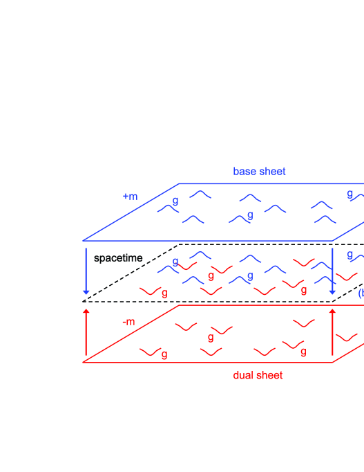
Figure 1: The double-sheeted spacetime. Gravitational waves propagate forwards in time on the base sheet (top), and propagate backwards in time on the dual sheet (bottom). Spacetime is a superposition of the dual sheet projected onto the base sheet (middle). The contribution to the curvature from the base sheet is positive, while the contribution from the dual sheet is negative, so that the resulting spacetime is essentially flat.

This kind of identification has been proposed by numerous authors in the past because of the striking number of similarities in physical properties between electrons and the charged, rotating, Kerr-Newman solution^?,?,?. Our model provides an explicit physical explanation for this identification, albeit without the need for a charge as, as we have shown, electric charge is an emergent property due to the motion of the fluid in the neighbourhood of the black hole, and is not an intrinsic physical property of the black hole itself.

We have noted that the two components of the relativistic fluid constituting the vacuum in our model are time-reversed versions of each other. This can be explained in the context of the maximally extended fast Kerr solution, which is the uncharged version of the model described in some detail by Arcos and Pereira^?. In Kerr-Schild coordinates, the fast Kerr solution takes the form^?,

$$ds^{2}=dt^{2}-dx^{2}-dy^{2}-dz^{2}-{2mr^{3}\over r^{4}+a^{2}z^{2}}\left({r(x\,dx+y\,dy)-a(x\,dy-y\,dx)\over r^{2}+a^{2}}+{z\,dz\over r}+dt\right)^{2}\,,$$ (49)

where $r$ is determined up to a sign by $r^{4}-(x^{2}+y^{2}+z^{2}-a^{2})r^{2}-a^{2}z^{2}=0$. Recalling that the maximal-extension of the fast Kerr geometry consists of two four-dimensional spacetime sheets, an incoming particle which crosses from the region with $r>0$ (which we will refer to as the ‘base’ sheet) through the wormhole throat at $r=0$, defined by the disc $x^{2}+y^{2}<a^{2},z=0$, will enter the second region with $r<0$ (which we will refer to as the ‘dual’ sheet). The dual sheet is identical to the base sheet but with the direction of propagation in time reversed. Similarly, any fluid particle in the dual sheet which passes through the wormhole throat at $r=0$ will emerge on the base sheet again with the direction of propagation in time reversed.

The physical picture this implies for a positively (negatively) charged particle is that it acts as a gravitational sink of fluid particles (antiparticles) in the base sheet, and these fluid particles (antiparticles) cross the Kerr wormhole throat and emerge from the dual sheet propagating backwards in time, so that the positively (negatively) charged particle simultaneously acts as a sink for fluid antiparticles (particles) in the dual sheet (see Figure 3). This implies that the 4-potential of a charged particle in §3.3 will have an equal contribution from both spacetime sheets on either side of the Kerr wormhole.

As explained by Chardin^?, particles travelling ‘backwards’ in time in the dual sheet will continue to interact with particles in the base sheet, and in particular, will appear to have the same physical properties as antiparticles travelling forwards in time on the base sheet. The base sheet and its dual will therefore appear to be superimposed onto a single four-dimensional spacetime, and to an external observer the process of absorption and reflection of a fluid particle will look not like a single infalling particle, but like a particle-antiparticle annihilation event occurring at the wormhole throat. This description is consistent with the analysis of Hadley^? who concludes that the failure of time-orientability of a spacetime region would be indistinguishable from a particle-antiparticle annihilation event.

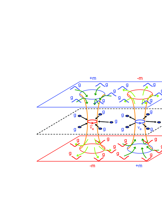
Figure 2: Neutrinos as sinks of gravitational waves. Neutrinos (antineutrinos) are formed from the gravitational collapse of gravitational waves in the dual (base) sheet, and have the spinorial geometry of a maximal fast Kerr wormhole throat connecting the base sheet to the dual sheet. The resulting dipole structure means that the isolated neutrinos and antineutrinos are massless but become polarised in a gravitational field. To an external observer, antineutrinos act as sinks of gravitational waves, while neutrinos act as sources.

An interaction between two charged particles can then be described by the exchange of a photon, which can be pictured as a twisted closed timelike loop formed by a fluid particle leaving the source particle, reflecting off the target particle and returning to the source, where it is once again reflected to return to its original position and time orientation (see Figure 4). This does not imply any causal inconsistency, as the process would merely have the appearance of a pair creation event at the source charge followed by a subsequent pair annihilation event at the target charge. As indicated in §3.8, whether the interaction results in an attraction or repulsion will depend on the nature (i.e. matter on antimatter) of the source and target charges, as well as the type of particles exchanged.

There exists a natural time-reversal symmetry in this model associated with the swapping of the base and dual spacetime sheets, which also exchanges the identity of matter and antimatter, and hence the sign of the gravitational mass (see Figure 1). This overall time-symmetric picture of charges and their interactions is reminiscent of the Wheeler-Feynman absorber theory^? of radiation, as well as Cramer’s transactional interpretation^? of quantum mechanics, and also of Hoyle and Narlikar’s action-at-a-distance^? cosmology. These connections will be explored in more detail in future work.

4.2 Neutrinos as Gravitational Dipoles

Hadley has shown^? that geon-like elementary particles in classical general relativity, of which our charged particles are particular examples, will naturally have the transformation properties of spinors if the spacetime manifold is not time-orientable. We conclude that the charged particles in our model are spinors, and we now formally identify them with electrons and positrons (see Figure 3).

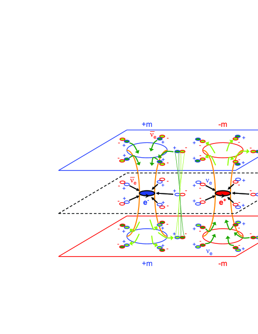
Figure 3: Electrons as sinks of antineutrinos. Electrons (positrons) are formed from the gravitational collapse of antineutrinos (neutrinos), and like neutrinos they have the geometry of the maximal fast Kerr solution. The antineutrinos (neutrinos) become polarised in the gravitational field of the charges, giving rise to the electron’s (positron’s) positive (negative) mass. In addition, the motion of the antineutrinos (neutrinos) in the neighbourhood of the Kerr wormhole throat give rise to the electron’s (positron’s) negative (positive) charge.

Given their fundamental nature, the fluid particles can be assumed to be ground state gravitational solitons formed from the collapse of intense gravitational waves, which are themselves nothing but ripples in spacetime. It is fairly well-established that gravitational waves of sufficient intensity can collapse to form black holes^?,?, so presumably there was enough energy in the early universe for these primordial black holes to be formed in enormous quantities. Having the geometry of the maximal fast Kerr solution, the fluid particles will themselves transform as spinors. Our earlier picture of fluid particles, which had assumed that each particle inhabits either the base sheet or its dual, will therefore need to be extended to allow each particle to have one component (i.e. the two regions on either side of the wormhole throat) on each spacetime sheet.

We know that the fluid particles are responsible, through their motion, for the appearance of charge, and so cannot be charged themselves. The only uncharged spinors observed in nature are the neutrinos, which do indeed fill spacetime, so it is natural to identify our fluid particles and antiparticles with neutrinos and antineutrinos respectively. The identification of these microscopic classical black holes with neutrinos seems particularly appropriate as Einstein and Rosen suggested the same identification themselves in their original paper^?. The two halves of the Einstein-Rosen bridge, one on each spacetime sheet, will have equal and opposite mass^?, and the neutrino therefore has the structure of a gravitational dipole (see Figure 2).

Because they are space-filling, the neutrinos effectively act like ‘pegs’ holding together the two spacetime sheets of the double-sheeted ‘Dirac-Milne’ universe recently described by Benoit-Lévy and Chardin^?. We saw in §3.4 that the propagation of electromagnetic waves could be represented by the oscillations of the positive and negative momentum particles out of phase. This implies that electromagnetic waves are described by the bounded oscillatory motion of neutrinos and antineutrinos, which is strongly reminiscent of the ‘neutrino theory of light’ that originated with the ideas of de Broglie^?. The neutrinos, then, are responsible for the physical vacuuum acting as a ‘luminiferous aether’.

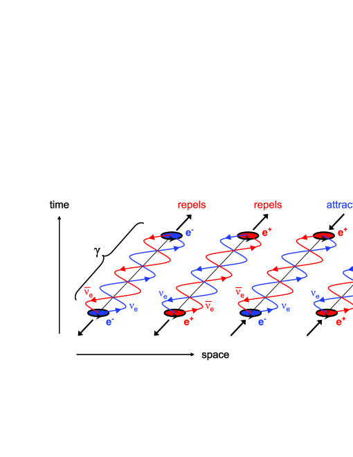
Figure 4: Like charges repel while opposite charges attract. Source electrons (positrons) emit neutrinos (antineutrinos) which are reflected back to the source by the target charge. The momentum transferred by the neutrinos cause target electrons (positrons) to be repelled (attracted), while antineutrinos cause target electrons (positrons) to be attracted (repelled). The photons look like twisted closed timelike loops formed by neutrino-antineutrino pairs travelling from source to target. The neutrino and antineutrino polarise each other, resulting in a van der Waals type interaction which is responsible for their oscillatory motion during the traversal from source to target.

The cancellation of the contributions from the base and dual components constituting the neutrino means that an isolated neutrino would be expected to have zero mass. However the gravitational dipole structure of the neutrino means that it will become polarised in the presence of a gravitational field in analogy with electrodynamics, and this polarisation will be manifested by a small relative translation of the two spacetime sheets with a magnitude of the same order as the radius of the ring singularity associated with the neutrino. As a result, the neutrino will be attracted towards any nearby massive body, irrespective of whether that body consists of matter or antimatter. This will give the neutrino the appearance of a small but finite mass of the same sign as the source.

This property can explain why electrons, which act as sinks of antineutrinos, appear to have mass, even though the antineutrinos themselves are massless. As the antineutrinos are attracted closer to the Kerr singularity, they become increasingly polarised, giving rise to the electron’s positive mass (see Figure 3). Similarly, positrons will attract neutrinos with opposite polarisation, giving rise to the positron’s negative mass.

The matter content of our model, which makes use of some of the results of §5, is summarised pictorially in Figures 1-4.

4.3 Exotic Cold Dark Matter and Modified Newtonian Dynamics

The polarisability of the neutrino means that in a matter-dominated region of the universe neutrinos will appear to have a small positive mass which would be compatible with recent observations. Despite their small apparent mass, it is natural to conjecture that the sheer number of neutrinos which fill spacetime could potentially account for the apparent missing dark matter in the universe.

The other significant physical consequence of the polarisability of the neutrino is that the physical vacuum will act like a gravitational dielectric or ‘digravitic’ in analogy with dielectrics in electrodynamics and this turns out to be the key to understanding the presence of modified Newtonian dynamics.

Indeed Blanchet showed in a recent paper^? that if there were to exist a space-filling ‘aether’ consisting of exotic dark matter particles which take the form of matter-antimatter dipoles (antimatter having negative mass), then this would satisfactorily explain the existence of MOND as a simple gravitational polarisation effect.

Clearly our model of the physical vacuum fits this description perfectly, with the neutrinos playing the role of the exotic matter which Blanchet describes. The implication of Blanchet’s results is that our model, which itself is based purely on Einstein’s general theory of relativity, actually predicts the existence of modified Newtonian dynamics.

To show how this works, following Blanchet, let us denote the gravitational potential by $U$. Then the gravitation field ${\bf g}$ associated with it is,

$${\bf g}=\nabla U\,.$$ (50)

Let the spatial vector ${\bf d}$ denote the separation between the positive and negative mass components of the (anti)neutrino, which will vary with the strength of the gravitational field. Then the dipole moment associated with each (anti)neutrino is,

$${\bf p}=m{\bf d}\,.$$ (51)

If the number density of dipoles is $n$, then the gravitational polarisation ${\bf P}$ will be,

$${\bf P}=n{\bf p}\,.$$ (52)

The positive gravitational mass component of the neutrino (we assume that all particles have positive inertial mass) will always be attracted by an external mass distribution consisting of ordinary matter, while the negative mass component will be repelled. The orientation of the dipole will then be such that the dipole moment ${\bf p}$, and hence the polarisation ${\bf P}$ points in the direction of the gravitational field ${\bf g}$.

The MOND equation in the form derivable from a non-relativistic Lagrangian is,

$$\nabla\cdot(\mu{\bf g})=-4\pi G\rho\,,$$ (53)

where $\rho$ is the density of ordinary matter, and the Milgrom function $\mu$ depends on the ratio $g/a_{0}$ where $g=|{\bf g}|$ is the magnitude of the gravitational field and $a_{0}$ is the constant acceleration scale. The MOND regime corresponds to the limit of weak gravity when $g\ll a_{0}$, in which case $\mu(g/a_{0})\approx g/a_{0}$. Similarly, in the strong field Newtonian regime when $g\gg a_{0}$, $\mu(g/a_{0})\rightarrow 1$, and we recover Newton’s law.

To make the analogy with electrostatics clear, note that the equation for an electric field in a dielectric medium is^?,

$$\nabla\cdot[(1+\chi_{e}){\bf E}]=\rho_{e}/\epsilon_{0}\,,$$ (54)

where $\chi_{e}$ denotes the electric susceptibility of the medium and depends on the magnitude of the electric field. Typically $\chi_{e}>0$, which corresponds to screening of the electric charges by the dielectric. The electric polarisation is then defined by,

$${\bf P}_{e}=\chi_{e}\epsilon_{0}{\bf E}\,,$$ (55)

In the case of gravitation, we can write the Milgrom function $\mu(g/a_{0})$ as,

$$\mu=1+\chi\,,$$ (56)

where $\chi=\chi(g/a_{0})$ is the gravitational susceptibility of the digravitic medium. The corresponding gravitational polarisation ${\bf P}$ is then,

$${\bf P}=-{\chi\over 4\pi G}\,{\bf g}\,,$$ (57)

Since in the gravitational case ${\bf P}$ is in the same direction as ${\bf g}$, the gravitational susceptibility $\chi$ must be negative,

$$\chi<0\,,$$ (58)

which is compatible with the MOND prediction that $0<\mu<1$ which requires that $-1<\chi<0$. The underlying reason for the negative gravitational susceptibility is simply the fact that like masses attract whereas like charges repel.

The equations of motion for the positive and negative mass components of the dipole are as follows,

$$m{d^{2}{\bf x}_{1}\over dt^{2}}=m{\bf g}({\bf x}_{1})-{\bf f}({\bf x}_{1}-{\bf x}_{2})\,,$$ (59)

$$m{d^{2}{\bf x}_{2}\over dt^{2}}=-m{\bf g}({\bf x}_{2})+{\bf f}({\bf x}_{1}-{\bf x}_{2})\,,$$ (60)

where ${\bf x}_{1}$ and ${\bf x}_{2}$ are the centre-of-mass positions of the positive and negative mass components respectively, and ${\bf f}({\bf x})$ is the force between them as a function of their separation. Let us transfer to new coordinates ${\bf x}={1\over 2}({\bf x}_{1}+{\bf x}_{2})$ representing the centre of the dipole and the dipole moment ${\bf p}=({\bf x}_{1}-{\bf x}_{2})$. Then after a first order Taylor expansion of ${\bf g}({\bf x})$, the evolution equation for the dipole is found to be,

$${d^{2}{\bf p}\over dt^{2}}=2m{\bf g}-2{\bf f}+{\mathcal{O}}(d^{2})\,,$$ (61)

while the equation of motion for the dipole in a gravitational field is,

$$2m{d^{2}{\bf x}\over dt^{2}}=({\bf p}\cdot\nabla)\nabla U+{\mathcal{O}}(d^{2})\,.$$ (62)

This tells us that the motion of the dipole is governed not by the strength of the gravitational field, but by its gradient, namely the tidal gravitational field. This means that the dipole will remain stationary in a constant gravitational field, and in a gravitational field outside a spherical massive body with potential $U\sim 1/r$, the dipole’s acceleration will be of the order of $1/r^{3}$ instead of the usual $1/r^{2}$ for an ordinary particle. Clearly the neutrinos seem to violate the equivalence principle, having an inertial mass of $2m$ and a gravitational mass of zero, and as such are good candidates for cold dark matter.

The question remains as to how the the dipole separation ${\bf d}$ varies with the field strength ${\bf g}$. Unlike Blanchet, we have no need to postulate a new internal force of non-gravitational origin, as we are well aware that what physically is happening when a neutrino is polarised is an attempt to rotate and pull the two poles into alignment with the external field. Small perturbations can be expected to follow a linear Hooke’s law pattern, as evidenced by the quasiharmonic motion describing the propagation of electromagnetic waves derived in (37), which represents a similar physical process. However there would be expected to be an asymptotic value beyond which the two poles can no longer be rotated or stretched, and so a reasonable parametric form for the dipole separation may be as follows,

$$d(g)=d_{0}\tanh(\alpha g)\,,$$ (63)

where $d_{0}$ is the dipole separation at saturation in the strong field limit, and the Hooke’s law ‘spring constant’ is given by $\alpha d_{0}$. From (57) and (63) the gravitational susceptibility $\chi$ would then take the form,

$$\chi=-4\pi Gnm{d\over g}\,,$$ (64)

so that the Milgrom function becomes approximately,

$$\mu(g/a_{0})\approx 1-4\pi Gnm{d_{0}\tanh(\alpha g)\over g}\,.$$ (65)

This has the correct property $\mu\rightarrow 1$ in the Newtonian regime when $g\gg a_{0}$. In the MOND regime, corresponding to the limit $g\rightarrow 0$, we require $\mu=g/a_{0}+{\mathcal{O}}(g^{2})$ in order to explain the flat rotation curves of galaxies. This fixes the value of $\alpha$ in (63),

$$\alpha={1-{g/a_{0}}\over 4\pi Gnmd_{0}}\,.$$ (66)

It seems unlikely that the true dependence of the dipole separation on the gravitational field strength will vary significantly from (63), and that any differences are likely to have limited physical consequences. The essential features that need to be present are that $d^{\prime}(g)/g$ in the zero field limit agrees with observations, and that $d/g\rightarrow 0$ in the strong field limit.

The physical picture we then have is as follows. When there is no gravitational field there is no polarisation, while at small but finite gravitational fields, the polarisation of the vacuum increases linearly with field strength, corresponding to the MOND regime. As the field strength increases further, the polarisation becomes saturated, reaching an asymptotic value, so that eventually the effects of vacuum polarisation become negligible in comparison with the external field and we return to the usual Newtonian regime. All of this appears to be a nontrivial consequence of classical general relativity without modification and without needing to introduce any new particles not already observed in nature. Indeed it appears that neutrinos and antineutrinos themselves can be identified as the ‘missing’ cold dark matter.

5 Antigravity and its Cosmological Consequences - Some Speculations

The possibility of negative mass in the context of general relativity was first discussed by Bondi^?. The article by Nieto and Goldman^? reviews theoretical arguments against the existence of antigravity. Nevertheless there has been a renewed interest in the possibility of antigravity^?,? on account of recent cosmological observations, including proposals for experimental verification^?,?. Chardin has argued that the existence of antigravity could explain the observed CP violation in the neutral kaon system^?. Moreover, antiparticles are predicted to have negative mass by the Dirac equation in relativistic quantum theory, and negative mass regions are actually rather commonplace in solutions of the Einstein equations in general relativity. These latter two facts seem in themselves to be sufficient reason to take the idea of antigravity quite seriously, rather than considering it to be an inconvenience or an embarrassment that must be explained away or brushed underneath the carpet and simply ignored.

We have shown here that antigravity must exist in the classical realm without invoking quantum mechanics, and that classical electrodynamics emerges directly from general relativity as a result. The presence of antigravity would naturally be expected to have consequences for some of the major outstanding issues in cosmology, and we very briefly discuss a number of such speculations here, most of which have already been put forward by others in different contexts.

5.1 Matter Dominated Regions and the Accelerating Expansion of the Universe

Perhaps the simplest consequence of antigravity is that matter will tend to clump together with matter and antimatter will tend to clump together with antimatter, but the two types of matter will repel. If we assume that there are comparable amounts of both matter and antimatter in the universe, the result will be region(s) of space which are matter dominated, and other region(s) which are antimatter dominated. In particular we appear to live in a matter-dominated region of the universe.

The repulsion between matter and antimatter dominated regions should in principle be observable, and indeed in the case of an open universe it would predict that the universe should expand at an accelerating rate, as is observed. This was mentioned by both Ripalda^? and Ni^?. Ni goes on to suggest that the supernovae observed to undergo acceleration may do so because they consist of antimatter and there is a repulsive force exerted upon them by inner galaxies consisting mainly of matter. He also proposes that increasing antimatter domination is responsible for the increasing rate of star formation at increasingly remote distances.

On the other hand it is a curious coincidence that the observed size of the universe is very close to the size that would be expected for a black hole of the same mass. If the observable universe is indeed enclosed within a non-traversable event horizon, or is otherwise bounded, then the result of antigravity would be a universe which undergoes cycles of expansion and contraction^?. If that is the case, then clearly we are in an accelerated expansion phase following an earlier deceleration, and this would agree with cosmological observations^?.

5.2 Gamma Ray Bursts

If matter and antimatter dominated regions do exist as antigravity would predict, then wherever the boundaries between the matter and antimatter dominated regions meet there will be some ‘rubbing together’ of the two, resulting in massive particle-antiparticle annihilation events which will give off huge bursts of electromagnetic radiation. This ‘cosmic lightning’ would be observed as gamma ray bursts. This explanation for the origin of gamma ray bursts has also been suggested by Ripalda^?. Ni^? further argues that the Earth is actually near the centre of a matter-dominated region based upon the observed isotropic distribution of gamma ray bursts.

5.3 The Cosmological Constant and Spacetime Curvature

Einstein’s general theory of relativity allows for the presence of a cosmological constant, but the value observed for $\Lambda$ is over 120 orders of magnitude smaller than that predicted from quantum vacuum effects. The tiny value observed for the cosmological constant can be explained at a fundamental level in the context of our model if all particles on the dual sheet have opposite energy to those on the base sheet. Because these particles always occur in pairs, their contribution to the vacuum energy will cancel, resulting in no net contribution to the cosmological constant. The small value of the cosmological constant could then be attributed to asymmetries between the base sheet and its dual, which in the context of our model can only be attributed to the presence of excess gravitational waves on the base sheet, namely those which do not collapse to form elementary particles such as neutrinos. Quiros^? has also suggested that there may exist two vacua, one gravitating and one antigravitating resulting in the mutual cancellation of their contributions to the cosmological constant. Alternatively, Moffat^? and Padmanabhan^? propose that fluctuations of vacuum energy density may be responsible for the observed cosmological constant.

The universe appears to be approximately flat with only a small positive curvature on cosmic scales. If energy is associated with curvature, then the same considerations above would explain the relative flatness of the universe, with the uncollapsed gravitational waves accounting for any small positive curvature that remains.

5.4 The Dirac-Milne Cosmology

The picture that emerges from our model is of a time-symmetric double-sheeted universe which treats matter and antimatter with an equal status. The compatibility of our model with the Wheeler-Feynman absorber theory of radiation suggests a reappraisal of the quasi-steady-state cosmology proposed by Hoyle and Narlikar^?.

More recently, Benoit-Lévy and Chardin, who also suggest the identification of elementary particles with the fast Kerr geometry, have examined the properties of a matter-antimatter-symmetric Milne spacetime filled with Kerr-Newman type particles, which they refer to as the ‘Dirac-Milne’ cosmology, and have found an excellent agreement with cosmological data without the high level of manual fine-tuning of parameters required with the $\Lambda$-CDM standard model^?. In particular, the Dirac-Milne cosmology appears to satisfy the cosmological tests for the age of the universe, big bang nucleosynthesis, type Ia supernovae data and even provides the degree scale for the first acoustic peak of the cosmological microwave background.

5.5 The Relationship Between Energy, Mass and Curvature

Our model predicts that there should be two superimposed spacetime sheets - the ‘base’ sheet, and the dual ‘sheet’. In the dual sheet, time goes in the opposite direction relative to the base sheet, so that an observer on the base sheet will observe a particle on the dual sheet to be travelling backwards in time. There must also be both particles and antiparticles on the same sheet, with the antiparticles travelling in the opposite direction in time to the particles.

However all of these identifications are relative to the particular frame of reference used, and different observers will in general disagree about what constitutes matter or antimatter and which sheet is the base sheet and which is its dual. Let us select one particular observer arbitrarily in order to establish a convention. According to that observer, there are four types of matter in existence, namely, matter on the base sheet ($B^{+}$), antimatter on the base sheet ($B^{-}$), matter on the dual sheet ($D^{+}$), and antimatter on the dual sheet ($D^{-}$).

Now, in addition to (a) the direction of propagation in time, there is associated with all of these types of matter, (b) a gravitational mass, (c) an inertial mass, (d) an energy, and (e) an apparent curvature of the surrounding spacetime. We would like to find out the sign of each of these five parameters for each of the four matter types in the context of our model. Based upon known observations we can come to the following conclusions:

• To account for Coulomb’s law in electrodynamics, it must be the case that particles and antiparticles on the same sheet have opposite gravitational mass. This has already been discussed in §3.8.

• To account for the zero mass of isolated neutrinos, which have a dipole structure, as well as for the existence of modified Newtonian dynamics, which is a consequence of gravitational polarisation of neutrinos, matter in the base sheet must have opposite gravitational mass to antimatter in the dual sheet.

• Because we live in a matter dominated part of the universe, and also indirectly from the observation that the universe is expanding at an accelerating rate, matter and antimatter in the same sheet must repel. This, together with their known sign of gravitational mass implies that the inertial mass of all particle types is positive.

• Because matter attracts matter and antimatter attracts antimatter, both of these must be associated with positive curvature in the same spacetime sheet as the observer.

• The near flatness of spacetime means that the total curvature is close to zero. This means that the curvature associated with matter and antimatter on the dual sheet must be negative and cancel the curvature due to matter and antimatter on the base sheet.

• Energy is released when matter and antimatter annihilates, so conservation of energy requires that matter and antimatter on the same sheet have the same sign of energy.

• The tiny value of the cosmological constant implies that the total energy of the vacuum must be very small, so that the energy of both matter and antimatter in the dual sheet must be negative.

Putting all of this information together, we finally arrive at the following table:

Particle type	$B^{+}$	$B^{-}$	$D^{+}$	$D^{-}$
Direction of time	$+$	$-$	$-$	$+$
Gravitational mass	$+$	$-$	$+$	$-$
Inertial mass	$+$	$+$	$+$	$+$
Energy	$+$	$+$	$-$	$-$
Spacetime curvature	$+$	$+$	$-$	$-$

We see from the table that energy is associated with spacetime curvature, and that neither of these are equivalent to either gravitational or inertial mass. Furthermore, we see that the principle of equivalence does not strictly hold for antimatter, as these have opposite (as opposed to equal) inertial and gravitational masses, requiring that the principle be generalised to describe antimatter correctly. The same conclusion was reached by Hossenfelder^?.

6 Discussion and Summary

We began with a simple description of the physical vacuum as a relativistic fluid in motion. We then showed that it was possible to derive classical electrodynamics in terms of the motion of a two-component matter-antimatter fluid with the electromagnetic 4-potential being identified with the time-averaged 4-momentum of the fluid. Charged particles act as gravitational sinks, and were therefore assumed to have a maximal fast Kerr geometry, which implies that spacetime is double-sheeted, and that antimatter has negative mass. The fluid particles were postulated to be neutral spinors formed from gravitational collapse of gravitational waves, and were identified as neutrinos. These have the same maximal fast Kerr geometry, which in turn implies that they are gravitational dipoles. Because the neutrinos are space-filling, this means that the vacuum must be gravitationally polarisable, and this was shown to be sufficient to explain the existence of modified Newtonian dynamics.

The entire model can be derived essentially from first principles from the general relativistic treatment of a space-filling fluid, and hence we have been able to show that classical electrodynamics and modified Newtonian dynamics are both non-trivial consequences of general relativity. The time and matter-antimatter symmetry of the model is compatible with the Wheeler-Feynman absorber theory of radiation, and hence Hoyle and Narlikar’s action-at-a-distance cosmology. The non-causal structure of the maximal fast Kerr solution gives rise to time-reversing process which suggest a relationship with Cramer’s transactional interpretation of quantum mechanics. It will be interesting to see whether this connection with quantum theory can be made explicit so that the model is able to provide a sound physical basis for quantum theory.

In terms of possible cosmological consequences we have discussed briefly how the model’s prediction of antigravity may help us to understand the accelerating expansion of the universe, the origin of gamma ray bursts, the smallness of the cosmological constant, the relationship between mass, energy and curvature, and also how the model may give rise to a Dirac-Milne universe which seems to agree well with cosmological data without the need for fine-tuning of parameters. Trayling and Baylis^? were able to derive the standard model gauge group in terms of Clifford algebra on a $7+1$-dimensional spacetime, so it would be of interest to see whether the standard model gauge group can similarly be derived from our model as a consequence of spacetime being double-sheeted.

7 Acknowledgements

I would like to thank Jan Bielawski, Steve Carlip, Steve Gull, Hugh Jones, Daryl McCullough, Abhas Mitra and Tom Roberts for useful discussions and feedback, and Roy Pike for his valuable support and encouragement. I would like to dedicate this paper to John Peach and Simon Altmann, my ex-tutors at Brasenose College.

8 References

References

- [1] L. Blanchet, Gravitational polarization and the MOND phenomenology, Class. Quant Grav. 24 (2007) 3529-3539.
- [2] J. D. Jackson, Classical Electrodynamics, 3rd edn., (John Wiley & Sons, 1998).
- [3] P. A. M. Dirac, A new classical theory of electrons, Proc. Roy. Soc. London, Ser. A 209 (1951) 291-296.
- [4] P. A. M. Dirac, Is there an aether?, Nature 168 (1951) 906-907, 169 (1952) 702.
- [5] L. D. Landau and E. M. Lifschitz, The Classical Theory of Fields, 4th revised English edn., Course of Theoretical Physics, Volume 2, p. 25, p.50 and p.299-301 (Pergamon Press, 1975).
- [6] R. L. Liboff, Kinetic Theory: Classical, Quantum and Relativistic Descriptions, 3rd edn., (Springer, 1998).
- [7] A. Einstein, Relativity: The Special and General Theory, reprint of 1st (1920) edn., (Dover Publications, 2001).
- [8] B. O’Neill, The Geometry of Kerr Black Holes, (A. K. Peters, 1995).
- [9] W. Israel, Source of the Kerr metric, Phys. Rev. D 2 (1970) 641-646.
- [10] H. I. Arcos and J. G. Pereira, Kerr-Newman solution as a Dirac particle, Gen. Rel. Grav. 36 (2004) 2411-2464.
- [11] A. Burinskii, Complex Kerr geometry, twistors and the Dirac electron, J. Phys. A 41 (2008) 164069.
- [12] S. W. Hawking and G. F. R. Ellis, The Large Scale Structure of Space-Time, (CUP, 1975).
- [13] G. Chardin, Motivations for antigravity in general relativity, Hyperfine Interactions 109 (1997) 83-94.
- [14] M. J. Hadley, The orientability of spacetime, Class. Quant. Grav. 17 (2000) 4187-4194.
- [15] J. A. Wheeler and R. P. Feynman, Interaction with the absorber as the mechanism of radiation, Rev. Mod. Phys. 17 (1945) 157-181.
- [16] J. G. Cramer, The transactional interpretation of quantum mechanics, Rev. Mod. Phys. 58 (1986) 647-687.
- [17] F. Hoyle and J. V. Narlikar, Cosmology and action-at-a-distance electrodynamics, Rev. Mod. Phys. 67 (1995) 113-155.
- [18] M. J. Hadley, Spin half in classical general relativity, Class. Quant. Grav. 17 (2000) 4187-4194.
- [19] A. M. Abrahams, Trapping a geon: Black hole formation by an imploding gravitational wave, Phys. Rev. D46 (1992) R4117-R4121.
- [20] M. Alcubierre, G. Allen, B. Bruegmann, G. Lanfermann, E. Seidel, W. Suen, and M. Tobias, Gravitational collapse of gravitational waves in 3D numerical relativity, Phys. Rev. D61 (2000) 041501.
- [21] A. D. Helfer, Do black holes radiate?, Rep. Prog. Phys. 66 (2003) 943-1008.
- [22] A. Einstein and N. Rosen, The particle problem in the general theory of relativity, Phys. Rev. 48 (1935) 73-77.
- [23] A. Benoit-Lévy and G. Chardin, Observational constraints of a symmetric Milne universe, Proc. 43rd Rencontres de Moriond 2008, arXiv:0811.2149.
- [24] L. de Broglie, Sur une analogie entre l’électron de Dirac et l’onde électromagnétique, Compt. Rend. Acad. Sci. 195 (1932) 536.
- [25] H. Bondi, Negative mass in general relativity, Rev. Mod. Phys. 29 423-428.
- [26] M. M. Nieto and T. Goldman, The arguments against ‘antigravity’ and the gravitational acceleration of antimatter, Phys. Rep. 205 (1991) 223-281.
- [27] S. Hossenfelder, Anti-gravitation, Phys. Lett. B636 (2006) 119-125.
- [28] G.-J. Ni, A new insight into the negative-mass paradox of gravity and the accelerating universe, Rel. Grav. Cosmol. 1 (2004) 123-136.
- [29] D. S. Hajdukovic, Testing existence of antigravity, gr-qc/0602041.
- [30] J. M. Ripalda, Space-time reversal antimatter, and antigravity in general relativity, gr-qc/9906012.
- [31] S. Hossenfelder, Cosmological consequences of anti-gravitation, gr-qc/0605083.
- [32] T. Padmanabhan, Understanding our universe: Current status and open issues, gr-qc/0503107.
- [33] I. Quiros, Symmetry relating gravity with antigravity: A possible resolution of the cosmological constant problem?, gr-qc/0411064.
- [34] J. W. Moffat, A solution to the cosmological constant problem, astro-ph/9606071.
- [35] T. Padmanabhan, Vacuum fluctuations of energy density can lead to the observed cosmological constant, Class. Quant. Grav. 22 (2005) L107-L110.
- [36] A. Benoit-Lévy and G. Chardin, Do we live in a ‘Dirac-Milne’ universe?, arXiv:0811.2149.
- [37] G. Trayling and W. E. Baylis, A geometric basis for the standard-model gauge group, J. Phys. A 34 (2001) 3309-3324.