Resolution limit in community detection

Abstract

Detecting community structure is fundamental to clarify the link between structure and function in complex networks and is used for practical applications in many disciplines. A successful method relies on the optimization of a quantity called modularity [Newman and Girvan, Phys. Rev. E 69, 026113 (2004)], which is a quality index of a partition of a network into communities. We find that modularity optimization may fail to identify modules smaller than a scale which depends on the total number $L$ of links of the network and on the degree of interconnectedness of the modules, even in cases where modules are unambiguously defined. The probability that a module conceals well-defined substructures is the highest if the number of links internal to the module is of the order of $\sqrt{2L}$ or smaller. We discuss the practical consequences of this result by analyzing partitions obtained through modularity optimization in artificial and real networks.

I Introduction

Community detection in complex networks has attracted a lot of attention in the last years (for a review see Newman:2004 ; Danon:2005 ). The main reason is that complex networks bara02 ; mendes03 ; Newman:2003 ; psvbook ; vitorep are made of a large number of nodes and that so far most of the quantitative investigations were focusing on statistical properties disregarding the roles played by specific subgraphs. Detecting communities (or modules) can then be a way to identify relevant substructures that may also correspond to important functions. In the case of the World Wide Web, for instance, communities are sets of Web pages dealing with the same topic Flake:2002 . Relevant community structures were also found in social networks Girvan:2002 ; Lusseau:2003 ; Adamic:2005 , biochemical networks Holme:2003 ; Guimera:2005 ; palla , the Internet Eriksen:2003 , food webs foodw , and in networks of sexual contacts sexcontact .

Loosely speaking a community is a subgraph of a network whose nodes are more tightly connected with each other than with nodes outside the subgraph. A decisive advance in community detection was made by Newman and Girvan Newman:2004b , who introduced a quantitative measure for the quality of a partition of a network into communities, the so-called modularity. This measure essentially compares the number of links inside a given module with the expected value for a randomized graph of the same size and degree sequence. If one takes modularity as the relevant quality function, the problem of community detection becomes equivalent to modularity optimization. The latter is not trivial, as the number of possible partitions of a network in clusters increases exponentially with the size of the network, making exhaustive optimization computationally unreachable even for relatively small graphs. Therefore, a number of algorithms have been devised in order to find a good optimization with the least computational cost. The fastest available procedures uses greedy techniques Newman:2004c ; Clauset:2004 and extremal optimization Duch:2005 , and are at present time the only algorithms capable to detect communities on large networks. More accurate results are obtained through simulated annealing Guimera:2004 ; Reichardt:2006 , although this method is computationally very expensive.

Modularity optimization seems thus to be a very effective method to detect communities, both in real and in artificially generated networks. The modularity itself has however not yet been thoroughly investigated and only a few general properties are known. For example, it is known that the modularity value of a partition does not have a meaning by itself, but only if compared with the corresponding modularity expected for a random graph of the same size Bornholdt:2006 , as the latter may attain very high values, due to fluctuations Guimera:2004 .

In this paper we focus on communities defined by modularity. We will show that modularity contains an intrinsic scale which depends on the number of links of the network, and that modules smaller than that scale may not be resolved, even if they were complete graphs connected by single bridges. The resolution limit of modularity actually depends on the degree of interconnectedness between pairs of communities and can reach values of the order of the size of the whole network. It is thus a priori impossible to tell whether a module (large or small), obtained through modularity optimization, is indeed a single module or a cluster of smaller modules. This result thus introduces some caveats in the use of modularity to detect community structure.

In Section II we recall the notion of modularity and discuss some of its properties. Section III deals with the problem of finding the most modular network with a given number of nodes and links. In Section IV we show how the resolution limit of modularity arises. In Section V we illustrate the problem with some artificially generated networks, and extend the discussion to real networks. Our conclusions are presented in Section VI.

II Modularity

The modularity of a partition of a network in modules can be written as Newman:2004b

$$Q=\sum_{s=1}^{m}\Big{[}\frac{l_{s}}{L}-\left(\frac{d_{s}}{2L}\right)^{2}\Big{]},$$ (1)

where the sum is over the $m$ modules of the partition, $l_{s}$ is the number of links inside module $s$, $L$ is the total number of links in the network, and $d_{s}$ is the total degree of the nodes in module $s$. The first term of the summands in Eq. (1) is the fraction of links inside module $s$; the second term instead represents the expected fraction of links in that module if links were located at random in the network (under the only constraint that the degree sequence coincides with that in the original graph). If for a subgraph ${\cal S}$ of a network the first term is much larger than the second, it means that there are many more links inside ${\cal S}$ than one would expect by random chance, so ${\cal S}$ is indeed a module. The comparison with the null model represented by the randomized network leads to the quantitative definition of community embedded in the ansatz of Eq. (1). We conclude that, in a modularity-based framework, a subgraph ${\cal S}$ with $l_{s}$ internal links and total degree $d_{s}$ is a module if

$$\frac{l_{s}}{L}-\left(\frac{d_{s}}{2L}\right)^{2}>0.$$ (2)

Let us express the number of links $l_{s}^{out}$ joining nodes of the module $s$ to the rest of the network in terms of $l_{s}$, i.e. $l_{s}^{out}=al_{s}$ with $a\geq 0$. So, $d_{s}=2l_{s}+l_{s}^{out}=(a+2)l_{s}$ and the condition (2) becomes

$$\frac{l_{s}}{L}-\left[\frac{(a+2)l_{s}}{2L}\right]^{2}>0,$$ (3)

from which, rearranging terms, one obtains

$$l_{s}<\frac{4L}{(a+2)^{2}}.$$ (4)

If $a=0$, the subgraph ${\cal S}$ is a disconnected part of the network and is a module if $l_{s}<L$ which is always true. If $a$ is strictly positive, Eq. (4) sets an upper limit to the number of internal links that ${\cal S}$ must have in order to be a module. This is a little odd, because it means that the definition of community implied by modularity depends on the size of the whole network, instead of involving a “local” comparison between the number of internal and external links of the module. For $a<2$ one has $2l_{s}>l_{s}^{out}$, which means that the total degree internal to the subgraph is larger than its external degree, i.e. $d^{in}_{s}>d^{out}_{s}$. The attributes “internal” and “external” here mean that the degree is calculated considering only the internal or the external links, respectively. In this case, the subgraph ${\cal S}$ would be a community according to the “weak” definition given by Radicchi et al. radicchi .

For $a<2$ the right-hand-side of inequality (4) is in the interval $[L/4,L]$. A subgraph of size $l_{s}$ would then be a community both within the modularity framework and according to the weak definition of Radicchi et al. if $a<2$ and $l_{s}$ is less than a quantity in the interval $[L/4,L]$. Sufficient conditions for which these constraints are always met are then

$$l_{s}<\frac{L}{4},a<2.$$ (5)

In Section IV we shall only consider modules of this kind.

According to Eq. (2), a partition of a network into actual modules would have a positive modularity, as all summands in Eq. (1) are positive. On the other hand, for particular partitions, one could bump into values of $Q$ which are negative. The network itself, meant as a partition with a single module, has modularity zero: in this case, in fact, $l_{1}=L$, $d_{1}=2L$, and the only two terms of the unique module in $Q$ cancel each other. Usually, a value of $Q$ larger than $0.3-0.4$ is a clear indication that the subgraphs of the corresponding partition are modules. However, the maximal modularity differs from a network to another and depends on the number of links of the network. In the next section we shall derive the expression of the maximal possible value $Q_{M}(L)$ that $Q$ can attain on a network with $L$ links. We will prove that the upper limit for the value of modularity for any network is $1$ and we will see why the modularity is not scale independent.

III The most modular network

In this section we discuss of the most modular network which will introduce naturally the problem of scales in modularity optimization. In Ref. Danon:2005 , the authors consider the interesting example of a network made of $m$ identical complete graphs (or ‘cliques’), disjoint from each other. In this case, the modularity is maximal for the partition of the network in the cliques and is given by the sum of $m$ equal terms. In each clique there are $l=L/m$ links, and the total degree is $d=2l$, as there are no links connecting nodes of the clique to the other cliques. We thus obtain

$$Q=m\Big{[}\frac{l}{L}-\left(\frac{2l}{2L}\right)^{2}\Big{]}=m\left(\frac{1}{m}-\frac{1}{m^{2}}\right)=1-\frac{1}{m},$$ (6)

which converges to $1$ when the number of cliques goes to infinity. We remark that for this result to hold it is not necessary that the $m$ connected components be cliques. The number of nodes of the network and within the modules does not affect modularity. If we have $m$ modules, we just need to have $L/m$ links inside the modules, as long as this is compatible with topological constraints, like connectedness. In this way, a network composed by $m$ identical trees (in graph theory, a forest) has the same maximal modularity reported in Eq. (6), although it has a far smaller number of links as compared with the case of the densely connected cliques (for a given number of nodes).

A further interesting question is how to design a connected network with $N$ nodes and $L$ links which maximizes modularity. To address this issue, we proceed in two steps: first, we consider the maximal value $Q_{M}(m,L)$ for a partition into a fixed number $m$ of modules; after that, we look for the number $m^{\star}$ that maximizes $Q_{M}(m,L)$.

Let us first consider a partition into $m$ modules. Ideally, to maximize the contribution to modularity of each module, we should reduce as much as possible the number of links connecting modules. If we want to keep the network connected, the smallest number of inter-community links must be $m-1$. For the sake of clarity, and to simplify the mathematical expressions (without affecting the final result), we assume instead that there are $m$ links between the modules, so that we can arrange the latter in the simple ring-like configuration illustrated in Fig. 1.

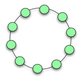
Figure 1: Design of a connected network with maximal modularity. The modules (circles) must be connected to each other by the minimal number of links.

The modularity of such a network is

$$Q=\sum_{s=1}^{m}\Big{[}\frac{l_{s}}{L}-\left(\frac{2l_{s}+2}{2L}\right)^{2}\Big{]},$$ (7)

where

$$\sum_{s=1}^{m}l_{s}=L-m.$$ (8)

It is easy to see that the expression of Eq. (7) reaches its maximum when all modules contain the same number of links, i.e. $l_{s}=l=L/m-1,\forall s=1,2,...,m$. The maximum is then given by

$$Q_{M}(m,L)=m\Big{[}\frac{L/m-1}{L}-\left(\frac{L/m}{L}\right)^{2}\Big{]}=1-\frac{m}{L}-\frac{1}{m}.$$ (9)

We have now to find the maximum of $Q_{M}(m,L)$ when the number of modules $m$ is variable. For this purpose we treat $m$ as a real variable and take the derivative of $Q_{M}(m,L)$ with respect to $m$

$$\frac{dQ_{M}(m,L)}{dm}=-\frac{1}{L}+\frac{1}{m^{2}}$$ (10)

which vanishes when $m=m^{\star}=\sqrt{L}$. This point indeed corresponds to the absolute maximum $Q_{M}(L)$ of the function $Q_{M}(m,L)$. This result coincides with the one found by the authors of Guimera:2004 for a one-dimensional lattice, but our proof is completely general and does not require preliminary assumptions on the type of network and modules.

Since $m$ is not a real number, the actual maximum is reached when $m$ equals one of the two integers closest to $m^{\star}$, but that is not important for our purpose, so from now on we shall stick to the real-valued expressions, their meaning being clear. The maximal modularity is then

$$Q_{M}(L)=Q_{M}(m^{\star},L)=1-\frac{2}{\sqrt{L}},$$ (11)

and approaches $1$ if the total number of links $L$ goes to infinity. The corresponding number of links in each module is $l=\sqrt{L}-1$. The fact that all modules have the same number of links does not imply that they have as well the same number of nodes. Again, modularity does not depend on the distribution of the nodes among the modules as long as the topological constraints are satisfied. For instance, if we assume that the modules are connected graphs, there must be at most $n=l+1=\sqrt{L}$ nodes in each module. The crucial point here is that modularity seems to have some intrinsic scale of order $\sqrt{L}$, which constrains the number and the size of the modules. For a given total number of nodes and links we could build many more than $\sqrt{L}$ modules, but the corresponding network would be less “modular”, namely with a value of the modularity lower than the maximum of Eq. (11). This fact is the basic reason why small modules may not be resolved through modularity optimization, as it will be clear in the next section.

IV The resolution limit

We analyze a network with $L$ links and with at least three modules, in the sense of the definition of formula (5) (Fig. 2). We focus on a pair of modules, ${\cal M}_{1}$ and ${\cal M}_{2}$, and distinguish three types of links: those internal to each of the two communities ($l_{1}$ and $l_{2}$, respectively), between ${\cal M}_{1}$ and ${\cal M}_{2}$ ($l_{int}$) and between the two communities and the rest of the network ${\cal M}_{0}$ ($l_{1}^{out}$ and $l_{2}^{out}$). In order to simplify the calculations we express the numbers of external links in terms of $l_{1}$ and $l_{2}$, so $l_{int}=a_{1}l_{1}=a_{2}l_{2}$, $l_{1}^{out}=b_{1}l_{1}$ and $l_{2}^{out}=b_{2}l_{2}$, with $a_{1},a_{2},b_{1},b_{2}\geq 0$. Since ${\cal M}_{1}$ and ${\cal M}_{2}$ are modules by construction, we also have $a_{1}+b_{1}\leq 2$, $a_{2}+b_{2}\leq 2$ and $l_{1},l_{2}<L/4$ (see Section II).

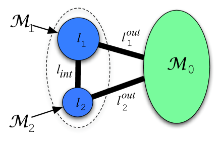
Figure 2: Scheme of a network partition into three or more modules. The two circles on the left picture two modules, the oval on the right reprensents the rest of the network ${\cal M}_{0}$, whose structure is arbitrary.

Now we consider two partitions $A$ and $B$ of the network. In partition $A$, ${\cal M}_{1}$ and ${\cal M}_{2}$ are taken as separate modules, and in partition $B$ they are considered as a single community. The split of the rest of the network is arbitrary but identical in both partitions. We want to compare the modularity values $Q_{A}$ and $Q_{B}$ of the two partitions. Since the modularity is a sum over the modules, the contribution of ${\cal M}_{0}$ is the same in both partitions and is denoted by $Q_{0}$. From Eq. (1) we obtain

$$Q_{A} = Q_{0}+\frac{l_{1}}{L}-\left[\frac{(a_{1}+b_{1}+2)l_{1}}{2L}\right]^{2}+\frac{l_{2}}{L}+$$ (12)

$$-\left[\frac{(a_{2}+b_{2}+2)l_{2}}{2L}\right]^{2};$$

$$Q_{B} = Q_{0}+\frac{l_{1}+l_{2}+a_{1}l_{1}}{L}+$$ (13)

$$-\left[\frac{(2a_{1}+b_{1}+2)l_{1}+(b_{2}+2)l_{2}}{2L}\right]^{2}.$$

The difference ${\Delta}Q=Q_{B}-Q_{A}$ is

$${\Delta}Q=\left[2La_{1}l_{1}-(a_{1}+b_{1}+2)(a_{2}+b_{2}+2)l_{1}l_{2}\right]/(2L^{2}).$$ (14)

As ${\cal M}_{1}$ and ${\cal M}_{2}$ are both modules by construction, we would expect that the modularity should be larger for the partition where the two modules are separated, i.e. $Q_{A}>Q_{B}$, which in turn implies ${\Delta}Q<0$. From Eq. (14) we see that ${\Delta}Q$ is negative if

$$l_{2}>\frac{2La_{1}}{(a_{1}+b_{1}+2)(a_{2}+b_{2}+2)}.$$ (15)

We see that if $a_{1}=a_{2}=0$, i.e. if there are no links between ${\cal M}_{1}$ and ${\cal M}_{2}$, the above condition is trivially satisfied. Instead, if the two modules are connected to each other, something interesting happens. Each of the coefficients $a_{1}$, $a_{2}$, $b_{1}$, $b_{2}$ cannot exceed $2$ and $l_{1}$ and $l_{2}$ are both smaller than $L/4$ by construction but can be taken as small as we wish with respect to $L$. In this way, it is possible to choose $l_{1}$ and $l_{2}$ such that the inequality of Eq. (15) is not satisfied. In such a situation we can have $\Delta Q>0$ and the modularity of the configuration where the two modules are considered as a single community is larger than the partition where the two modules are clearly identified. This implies that by looking for the maximal modularity, there is the risk to miss important structures at smaller scales. To give an idea of the size of $l_{1}$ and $l_{2}$ at which modularity optimization could fail, we consider for simplicity the case in which ${\cal M}_{1}$ and ${\cal M}_{2}$ have the same number of links, i.e. $l_{1}=l_{2}=l$. The condition on $l$ for the modularity to miss the two modules also depends on the fuzziness of the modules, as expressed by the values of the parameters $a_{1}$, $a_{2}$, $b_{1}$, $b_{2}$. In order to find the range of potentially “dangerous” values of $l$, we consider the two extreme cases in which

• the two modules have a perfect balance between internal and external degree ($a_{1}+b_{1}=2$, $a_{2}+b_{2}=2$), so they are on the edge between being or not being communities, in the weak sense defined in  radicchi ;

• the two modules have the smallest possible external degree, which means that there is a single link connecting them to the rest of the network and only one link connecting each other ($a_{1}=a_{2}=b_{1}=b_{2}=1/l$).

In the first case, the maximum value that the coefficient of $L$ can take in Eq. (15) is $1/4$, when $a_{1}=a_{2}=2$ and $b_{1}\approx 0$, $b_{2}\approx 0$, so we obtain that Eq. (15) may not be satisfied for

$$l<l_{R}^{max}=\frac{L}{4},$$ (16)

which is a scale of the order of the size of the whole network. In this way, even a pair of large communities may not be resolved if they share enough links with the nodes outside them (in this case we speak of “fuzzy” communities). A more striking result emerges when we consider the other limit, i.e. when $a_{1}=a_{2}=b_{1}=b_{2}=1/l$. In this case it is easy to check that Eq. (15) is not satisfied for values of the number of links inside the modules satisfying

$$l<l_{R}^{min}=\sqrt{\frac{L}{2}}.$$ (17)

If we now assume that we have two (interconnected) modules with the same number of internal links $l<l_{R}^{min}<l_{R}^{max}$, the discussion above implies that the modules cannot be resolved through modularity optimization, not even if they were complete graphs connected by a single link. As we have seen from Eq. (16), it is possible to miss modules of larger size, if they share more links with the rest of the network (and with each other). For $l_{1}\neq l_{2}$ the conclusion is similar but the scales $l_{R}^{min,max}$ are modified by simple factors.

V Consequences

We begin with a very schematic example, for illustrative purposes. In Fig. 3(A) we show a network consisting of a ring of cliques, connected through single links. Each clique is a complete graph $K_{m}$ with $m$ nodes and has $m(m-1)/2$ links. If we assume that there are $n$ cliques, with $n$ even, the network has a total of $N=nm$ nodes and $L=nm(m-1)/2+n$ links.

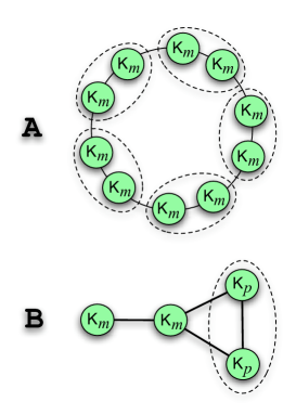
Figure 3: (A) A network made out of identical cliques (which are here complete graphs with $m$ nodes) connected by single links. If the number of cliques is larger than about $\sqrt{L}$, modularity optimization would lead to a partition where the cliques are combined into groups of two or more (represented by a dotted line). (B) A network with four pairwise identical cliques (complete graphs with $m$ and $p<m$ nodes, respectively); if $m$ is large enough with respect to $p$ (e.g. $m=20$, $p=5$), modularity optimization merges the two smallest modules into one (shown with a dotted line).

The network has a clear modular structure where the communities correspond to single cliques and we expect that any detection algorithm should be able to detect these communities. The modularity $Q_{single}$ of this natural partition can be easily calculated and equals

$$Q_{single}=1-\frac{2}{m(m-1)+2}-\frac{1}{n}.$$ (18)

On the other hand, the modularity $Q_{pairs}$ of the partition in which pairs of consecutive cliques are considered as single communities (as shown by the dotted lines in Fig. 3(A)) is

$$Q_{pairs}=1-\frac{1}{m(m-1)+2}-\frac{2}{n}.$$ (19)

The condition $Q_{single}>Q_{pairs}$ is satisfied if and only if

$$m(m-1)+2>n.$$ (20)

In this example, $m$ and $n$ are independent variables and we can choose them such that the inequality of formula (20) is not satistied. For instance, for $m=5$ and $n=30$, $Q_{single}=0.876$ and $Q_{pairs}=0.888>Q_{single}$. An efficient algorithm looking for the maximum of the modularity would find the configuration with pairs of cliques and not the actual modules. The difference $Q_{pairs}-Q_{single}$ would be even larger if $n$ increases, for $m$ fixed.

The example we considered was particularly simple and hardly represents situations found in real networks. However, the initial configuration that we considered in the previous section (Fig. 2) is absolutely general, and the results make us free to design arbitrarily many networks with obvious community structures in which modularity optimization does not recognize (some of) the real modules. Another example is shown in Fig. 3(B). The circles represent again cliques, i.e. complete graphs: the two on the left have $m$ nodes each, the other two $p<m$ nodes. If we take $m=20$ and $p=5$, the maximal modularity of the network corresponds to the partition in which the two smaller cliques are merged [as shown by the dotted line in Fig. 3(B)]. This trend of the optimal modularity to group small modules has already been remarked in Muff:2005 , but as a result of empirical studies on special networks, without any complete explanation.

In general, we cannot make any definite statement about modules found through modularity optimization without a method which verifies whether the modules are indeed single communities or a combination of communities. It is then necessary to inspect the structure of each of the modules found. As an example, we take the network of Fig. 3(A), with $n=30$ identical cliques, where each clique is a $K_{m}$ with $m=5$. As already said above, modularity optimization would find modules which are pairs of connected cliques. By inspecting each of the modules of the ‘first generation’ (by optimizing modularity, for example), we would ultimately find that each module is actually a set of two cliques.

We thus have seen that modules identified through modularity optimization may actually be combinations of smaller modules. During the process of modularity optimization, it is favorable to merge connected modules if they are sufficiently small.

We have seen in the previous Section that any two interconnected modules, fuzzy or not, are merged if the number of links inside each of them does not exceed $l_{R}^{min}$. This means that the largest structure one can form by merging a pair of modules of any type (including cliques) has at least $2l_{R}^{min}$ internal links. By reversing the argument, we conclude that if modularity optimization finds a module $\cal S$ with $l_{S}$ internal links, it may be that the latter is a combination of two or more smaller communities if

$$l_{S}<2l_{R}^{min}=\sqrt{2L}.$$ (21)

This example is an extreme case, in which the internal partition of $\cal S$ can be arbitrary, as long as the pieces are modules in the sense discussed in Section  II. Under the condition (21), the module could in principle be a cluster of loosely interconnected complete graphs.

On the other hand, the upper limit of $l_{S}$ can be much larger than $\sqrt{2L}$, if the substructures are on average more interconnected with each other, as we have seen in Section IV. In fact, fuzzy modules can be combined with each other even if they contain many more than $l_{R}^{min}$ links. The more interconnected the modules, the larger will be the resulting supermodule. In the extreme case in which all submodules are very fuzzy, the size $l_{S}$ of the supermodule could be in principle as large as that of the whole network, i.e. $l_{S}<L$. This result comes from the extreme case where the network is split in two very fuzzy communities, with $L/4$ internal links each and $L/2$ between them. By virtue of Eq. (16), it is favorable (or just as good) to merge the two modules and the resulting structure is the whole network. This limit $l_{S}<L$ is of course always satisfied but suggests here that it is important to carefully analyze all modules found through modularity optimization, regardless of their size.

The probability that a very large module conceals substructures is however small, because that could only happen if all hidden submodules are very fuzzy communities, which is unlikely. Instead, modules with a size $l_{S}\sim\sqrt{2L}$ or smaller can result from an arbitrary merge of smaller structures, which may go from loosely interconnected cliques to very fuzzy communities. Modularity optimization is most likely to fail in these cases.

In order to illustrate this theoretical discussion, we analyze five examples of real networks:

1. the transcriptional regulation network of Saccharomyces cerevisiae (yeast);

2. the transcriptional regulation network of Escherichia coli;

3. a network of electronic circuits;

4. a social network;

5. the neural network of Caenorhabditis Elegans.

We downloaded the lists of edges of the first four networks from Uri Alon’s Website alonwebsite , whereas the last one was downloaded from the WebSite of the Collective Dynamics Group at Columbia University colweb .

In the transcriptional regulation networks, nodes represent operons, i.e. groups of genes that are transcribed on to the same mRNA and an edge is set between two nodes A and B if A activates B. These systems have been previously studied to identify motifs in complex networks alon . There are $688$ nodes, $1,079$ links for yeast, $423$ nodes and $519$ links for E. coli. Electronic circuits can be viewed as networks in which vertices are electronic components (like capacitors, diodes, etc.) and connections are wires. Our network maps one of the benchmark circuits of the so-called ISCAS’89 set; it has $512$ nodes, $819$ links. In the social network we considered, nodes are people of a group and links represent positive sentiments directed from one person to another, based on questionnaires: it has $67$ nodes and $182$ links. Finally, the neural network of C. elegans is made of $306$ nodes (neurons), connected through $2,345$ links (synapsis, gap junctions). We remark that most of these networks are directed, here we considered them as undirected.

First, we look for the modularity maximum by using simulated annealing. We adopt the same recipe introduced in Ref. Guimera:2005 , which makes the optimization procedure very effective. There are two types of moves to pass from a network partition to the next: individual moves, where a single node is passed from a community to another, and collective moves, where a pair of communities is merged into a single one or, vice versa, a community is split into two parts. Each iteration at the same temperature consists of a succession of $N^{2}$ individual and $N$ collective moves, where $N$ is the total number of nodes of the network. The initial temperature $T$ and the temperature reduction factor $f$ are arbitrarily tuned to find the highest possible modularity: in most cases we took $T\sim 1$ and $f$ between $0.9$ and $0.99$.

We found that all networks are characterized by high modularity peaks, with $Q_{max}$ ranging from $0.4022$ (C. elegans) to $0.7519$ (E. coli). The corresponding optimal partitions consist of $9$ (yeast), $27$ (E. coli), $11$ (electronic), $10$ (social) and $4$ (C. elegans) modules (for E. coli our results differ but are not inconsistent with those obtained in Guimera:2005 for a slighly different database; these differences however do not affect our conclusions). In order to check if the communities have a substructure, we used again modularity optimization, by constraining it to each of the modules found. In all cases, we found that most modules displayed themselves a clear community structure, with very high values of $Q$. The total number of submodules is $57$ (yeast), $76$ (E. coli), $70$ (electronic), $21$ (social) and $15$ (C. elegans), and is far larger than the corresponding number at the modularity peaks. The analysis of course is necessarily biased by the fact that we neglect all links between the original communities, and it may be that the submodules we found are not real modules for the original network. In order to verify that, we need to check whether the condition of Eq. (2) is satisfied or not for each submodule and we found that it is the case. A further inspection of the communities found through modularity optimization thus reveals that they are, in fact, clusters of smaller modules. The modularity values corresponding to the partitions of the networks in the submodules are clearly smaller than the peak modularities that we originally found through simulated annealing (see Table 1). By restricting modularity optimization to a module we have no guarantee that we accurately detect its substructure and that this is a safe way to proceed. Nevertheless, we have verified that all substructures we detected are indeed modules, so our results show that the search for the modularity optimum is not equivalent to the detection of communities defined through Eq. (2).

network	$\#$ modules ($Q_{max}$)	total $\#$ of modules ($Q$)
Yeast	9 (0.7396)	57 (0.6770)
E. Coli	27 (0.7519)	76 (0.6615)
Electr. circuit	11 (0.6701)	70 (0.6401)
Social	10 (0.6079)	21 (0.5316)
C. elegans	4 (0.4022)	15 (0.3613)

Table 1: Results of the modularity analysis on real networks. In the second column, we report the number of modules detected in the partition obtained for the maximal modularity. These modules however contain submodules and in the third column we report the total number of submodules we found and the corresponding value of the modularity of the partition, which is lower than the peak modularity initially found.

The networks we have examined are fairly small but the problem we pointed out can only get worse if we increase the network size, especially when small communities coexist with large ones and the module size distribution is broad, which happens in many cases Clauset:2004 ; Danon:2006 . As an example, we take the recommendation network of the online seller Amazon.com. While buying a product, Amazon recommends items which have been purchased by people who bought the same product. In this way it is possible to build a network in which the nodes are the items (books, music), and there is an edge between two items $A$ and $B$ if $B$ was frequently purchased by buyers of $A$. Such a network was examined in Ref. Clauset:2004 and is very large, with $409,687$ nodes and $2,464,630$ edges. The authors analyzed the community structure by greedy modularity optimization which is not necessarily accurate but represents the only strategy currently available for large networks. They identified $1,684$ communities whose size distribution is well approximated by a power law with exponent $2$. From the size distribution, we estimated that over $95\%$ of the modules have sizes below the limit of Eq. (21), which implies that basically all modules need to be further investigated.

VI Conclusions

In this article we have analyzed in detail modularity and its applicability to community detection. We have found that the definition of community implied by modularity is actually not consistent with its optimization which may favour network partitions with groups of modules combined into larger communities. We could say that, by enforcing modularity optimization, the possible partitions of the system are explored at a coarse level, so that modules smaller than some scale may not be resolved. The resolution limit of modularity does not rely on particular network structures, but only on the comparison between the sizes of interconnected communities and that of the whole network, where the sizes are measured by the number of links.

The origin of the resolution scale lies in the fact that modularity is a sum of terms, where each term corresponds to a module. Finding the maximal modularity is then equivalent to look for the ideal tradeoff between the number of terms in the sum, i.e. the number of modules, and the value of each term. An increase of the number of modules does not necessarily correspond to an increase in modularity because the modules would be smaller and so would be each term of the sum. This is why for some characteristic number of terms the modularity has a peak. The problem is that this “optimal” partition, imposed by mathematics, is not necessarily correlated with the actual community structure of the network, where communities may be very heterogeneous in size, especially if the network is large.

Our result implies that modularity optimization might miss important substructures of a network, as we have confirmed in real world examples. From our discussion we deduce that it is not possible to exclude that modules of virtually any size may be clusters of modules, although the problem is most likely to occur for modules with a number of internal links of the order of $\sqrt{2L}$ or smaller. For this reason, it is crucial to check the structure of all detected modules, for instance by constraining modularity optimization on each single module, a procedure which is not safe but may give useful indications.

The fact that quality functions such as the modularity have an intrinsic resolution limit calls for a new theoretical framework which focuses on a local definition of community, regardless of its size. Quality functions are still helpful, but their role should be probably limited to the comparison of partitions with the same number of modules.

Acknowledgments.– We thank A. Barrat, C. Castellano, V. Colizza, A. Flammini, J. Kertész and A. Vespignani for enlightening discussions and suggestions. We also thank U. Alon for providing the network data.

References

- (1) M. E. J. Newman, Eur. Phys. J. B 38, 321-330 (2004).
- (2) L. Danon, A. Díaz-Guilera, J. Duch and A. Arenas, J. Stat. Mech., p. P09008, (2005).
- (3) A.-L. Barabási and R. Albert, Rev. Mod. Phys. 74, 47-97 (2002).
- (4) S. N. Dorogovtsev and J. F. F. Mendes, Evolution of Networks: from biological nets to the Internet and WWW (Oxford University Press, Oxford 2003).
- (5) M. E. J. Newman, SIAM Review 45, 167-256 (2003).
- (6) R. Pastor-Satorras and A. Vespignani, Evolution and structure of the Internet: A statistical physics approach (Cambridge University Press, Cambridge, 2004).
- (7) S. Boccaletti, V. Latora, Y. Moreno, M. Chavez and D.-U. Hwang, Phys. Rep. 424, 175-308 (2006).
- (8) G. W. Flake, S. Lawrence, C. Lee Giles and F. M. Coetzee, IEEE Computer 35(3), 66-71 (2002).
- (9) M. Girvan and M. E. J. Newman, Proc. Natl. Acad. Sci. 99, 7821-7826 (2002).
- (10) D. Lusseau and M. E. J. Newman, Proc. R. Soc. London B 271, S477-S481 (2004).
- (11) L. Adamic and N. Glance, Proc. Int. Workshop on Link Discovery, 36-43 (2005).
- (12) P. Holme, M. Huss and H. Jeong, Bioinformatics 19, 532 (2003).
- (13) R. Guimerà and L. A. N. Amaral, Nature 433, 895-900 (2005).
- (14) G. Palla, I. Derényi, I. Farkas and T. Vicsek, Nature 435, 814-818 (2005).
- (15) K. Eriksen, I. Simonsen, S. Maslov and K. Sneppen, Phys. Rev. Lett. 90, 148701 (2003).
- (16) S. L. Pimm, Theor. Popul. Biol. 16, 144 (1979); A. E. Krause, K. A. Frank, D. M. Mason, R. E. Ulanowicz and W. W. Taylor, Nature 426, 282 (2003).
- (17) G. P. Garnett, J. P. Hughes, R. M. Anderson, B. P. Stoner, S. O. Aral, W. L. Whittington, H. H. Handsfield and K. K. Holmes, Sexually Transmitted Diseases 23, 248-257 (1996); S. O. Aral, J. P. Hughes, B. P. Stoner, W. L. Whittington, H. H. Handsfield, R. M. Anderson and K. K. Holmes, American Journal of Public Health 89, 825-833 (1999).
- (18) M. E. J. Newman and M. Girvan, Phys. Rev. E 69, 026113 (2004).
- (19) M. E. J. Newman, Physical Review E 69, 066133 (2004).
- (20) A. Clauset, M. E. J. Newman and C. Moore, Phys. Rev. E 70, 066111 (2004).
- (21) J. Duch and A. Arenas, Phys. Rev. E 72, 027104 (2005).
- (22) R. Guimerà, M. Sales-Pardo and L. A. N. Amaral, Phys. Rev. E 70, 025101(R) (2004).
- (23) J. Reichardt and S. Bornholdt, preprint cond-mat/0603718 (2006).
- (24) J. Reichardt and S. Bornholdt, preprint cond-mat/0606220 (2006).
- (25) F. Radicchi, C. Castellano, F. Cecconi, V. Loreto and D. Parisi, Proc. Natl. Acad. Sci. 101, 2658-2663 (2004).
- (26) S. Muff, F. Rao, A. Caflisch, Phys. Rev. E 72, 056107 (2005).
- (27) L. Danon, A. Díaz-Guilera and A. Arenas, preprint physics/0601144 (2006).
- (28) R. Milo, S. Shen-Orr, S. Itzkovitz, N. Kashtan, D. Chklovskii and U. Alon, Science 298, 824-827 (2002).
- (29) http://www.weizmann.ac.il/mcb/UriAlon/.
- (30) http://cdg.columbia.edu/.