Rogue decoherence in the formation of a macroscopic atom-molecule superposition

Abstract

We theoretically examine two-color photoassociation of a Bose-Einstein condensate, focusing on the role of rogue decoherence in the formation of macroscopic atom-molecule superpositions. Rogue dissociation occurs when two zero-momentum condensate atoms are photoassociated into a molecule, which then dissociates into a pair of atoms of equal-and-opposite momentum, instead of dissociating back to the zero-momentum condensate. As a source of decoherence that may damp quantum correlations in the condensates, rogue dissociation is an obstacle to the formation of a macroscopic atom-molecule superposition. We study rogue decoherence in a setup which, without decoherence, yields a macroscopic atom-molecule superposition, and find that the most favorable conditions for said superposition are a density $\rho\sim 10^{12}\,{\rm cm}^{-3}$ and temperature $T\sim 10^{-10}\,{\rm K}$.

I Introduction

Since the famous thought experiment by Schrödinger Schrödinger (1935), macroscopic superpositions have been a part of quantum folklore that have annoyed specialists of the field. Schrödinger considered a cat that was sealed into a steel chamber with a diabolic device that consists of a small amount of radioactive material and a Geiger counter that was attached to a hammer device. If one radioactive nucleus would decay, then the Geiger counter would trigger the hammer device, and the hammer device would scrap a small bottle of Prussic acid which kills the cat. If the problem is studied strictly quantum mechanically, from outside the steel chamber, one finds that after a while the cat would be in a superposition state of alive and dead. If the cat would be in the statistical mixture of being alive or dead, the situation would not differ much from, e.g., tossing a coin with the probability of 0.5 for heads or tails. In a classical model, we do not yet know the outcome, but the state of the cat (coin) is either alive or dead (heads or tails), even before the measurement. The quantum cat (coin) behaves differently, with laws that allow superpositions between the outcome alive and outcome dead (heads and tails). Hence, rather than certain alive or certain dead (heads or tails) before the measurement, there must be quantum correlations between the the two outcomes.

For Schrödinger, the reason for putting the cat in the experimental spotlight was obvious. The absurd outcome of the experiment illustrated that, if the outcome was a result of treating everything–including the cat–strictly quantum mechanically, something was wrong, if not in the theory itself, then at least in the understanding quantum mechanics. As previous decoherence studies have shown Zurek (1982); Caldeira & Leggett (1983); Unruh et Zurek (1989); Zurek (1991); Hu et al. (1992); Anglin et al. (1995); Brune et al. (1996), one should be wary of too many oversimplifications and approximations. The environment of the cat should also be modelled, not only a point-like cat in a vacuum. The interaction between the cat and the environment induces decoherence that damps quantum correlations out of the cat, resulting in a classical statistical mixture of living and dead cat. In other words, the cat is too macroscopic to be in a superposition state. But what, then, is the upper limit of macroscopicity for a superposition state?

Recent studies Ruostekoski et al. (1998); Cirac et al. (1998); Gordon and Savage (1999); Dalvit, Dziarmaga, and Zurek (2000); Calsamiglia, Mackie & Suominen (2001); Huang et Moore (2005) have pointed out that the macroscopicity question can perhaps be addressed with Bose-Einstein condensates. References Ruostekoski et al. (1998); Cirac et al. (1998); Gordon and Savage (1999); Dalvit, Dziarmaga, and Zurek (2000) consider superpositions of two-component atomic condensates, while dynamical creation of a macroscopic superposition between atomic and molecular condensates via photoassociation Calsamiglia, Mackie & Suominen (2001) or Feshbach resonance Huang et Moore (2005) has also been studied. The work herein is a follow-up study of Calsamiglia, Mackie & Suominen (2001), one that includes dissociative damping of quantum correlations. In particular, we consider a macroscopic atom-molecule superposition created in a two step process: first, a joint atom-molecule condensate is created from an initial atomic condensate with strong photoassociation (compared to the s-wave collisional interaction); second, the photoassociation coupling is reduced, and a macroscopic atom-molecule superposition is created via strong s-wave collisions; observation is based on a Rabi-like oscillation of the system between the initial joint atom-molecule condensate and the corresponding macroscopic superposition. Here the main concern is to determine whether or not dissociative decoherence prohibits the photoassociative formation of a macroscopic atom-molecule superposition.

Photoassociation occurs when two atoms absorb a photon, thereby jumping from the two-atom continuum to a bound molecular state Drummond, Kheruntsyan, and He (1998); Julienne et al. (1998); Weiner et al. (1999); Javanainen et Mackie (1999); Heinzen et al. (2000); Kostrun et al. (2000); Hope et Olsen (2001); Vardi et al. (2001); Goral et al. (2001); Holland et al. (2001); Javanainen et Mackie (2002). For initially quantum-degenerate atoms, there is an analogy in nonlinear optics: photoassociation is formally identical to second-harmonic generated photons Walls et Tindle (1972), while s-wave collisions between the particles correspond to amplitude dispersion Yurke et Stoler (1986); in each case, the inherent non-linearity entangles the particles, and potentially leads to macroscopic superpositions. In photoassociation, however, the molecular state is excited and may spontaneously decay to molecular levels outside the system; also, the molecule may dissociate either back to the atomic condensate, or to a pair of noncondensate atoms of equal and opposite momentum via rogue Javanainen et Mackie (1999); Kostrun et al. (2000); Javanainen et Mackie (2002); Mackie (2003), i.e., unwanted Goral et al. (2001); Holland et al. (2001); NAI03 , photodissociation. These problems can be overcome by coupling the excited molecular state with a stable molecular state using a second laser. In this two-color photoassociation, the population loss via the excited molecular state can be made small by applying suitably large intermediate detunings. Nevertheless, decay of the quantum coherence is still possible, even if the populations are unaffected, and it is this possibility that warrents an invstigation of rogue dissociation in macroscopic atom-molecule superpositions.

The possible creation of a macroscopic atom-molecule superposition using photoassociation was reported in Calsamiglia et al. Calsamiglia, Mackie & Suominen (2001). Although lacking decoherence effects, the results were promising and, moreover, Ref. Calsamiglia, Mackie & Suominen (2001) is an interesting starting point for our study for several other reasons: the possibility of a superposition of atom-molecule condensates is tempting in itself, since atoms and molecules are different objects; the whole dynamical process of creating the superposition state can be modelled; the dissociation environment can be modelled in a straightforward manner. In Ref. Huang et Moore (2005) the dynamical approach has been used but, instead of photoassociation, the macroscopic superposition state was created with the help of a magnetic field and Feshbach resonance. The main source of decoherence was the laser-field induced interaction between atoms and the electromagnetic vacuum; however, the role of decoherence due to the coupling between magnetic field modes and the condensate is unclear. Also, the study of Ref. Calsamiglia, Mackie & Suominen (2001) considers the case of superposition very loosely. One cannot prove that the state is a superposition state by using probability distributions only. Of course, the possibility of a Rabi-like oscillations to and from the macroscopic superposition Calsamiglia, Mackie & Suominen (2001), on which observation is based, is more likely in the presence of quantum coherence; but, close revivals may also occur for nearly statistical mixtures. In all rigor, a detailed study of superposition states should include the off-diagonal elements of the density matrix, including the possibility of dissociative decoherence.

Hence, we focus on decoherence due to the second order term of the master equation for the condensate modes in the perturbation theory (anomalous quantum correlations induced by the first order term have been discussed elsewhere Mackie (2003)). Our results are roughly summarized as follows. In general, the decoherence timescale $\tau_{d}$ should be longer than the particular interaction timescale $\tau_{i}$, and thus macroscopic superpositions are possible only if the condition

$$\xi_{d}=\frac{\tau_{d}}{\tau_{i}}>>1$$ (1)

is fulfilled. Our scheme is divided into two phases in which different interactions are dominant. In phase $I$, we use photoassociation that is strong compared to collisions to drive the initial atomic condensate into a particular joint atom-molecule which serves as an initial state for the superposition engineering. Thus, the time scale $\tau_{i}$ is the photoassociation timescale. In phase $II$, the intensity of photoassociation laser is turned down, and dominant collisions between condensate particles drive the system into a macroscopic atom-molecule superposition. The interaction timescale is then the collision timescale. With the given simulation parameters we can express the coherence condition as

$$\xi_{d}=\frac{P_{I(II)}}{\rho[{\rm m^{3}}](2n^{2}+2n+1)},$$ (2)

where $P_{I}=2.712057\times 10^{10}$, $P_{II}=2.408246\times 10^{10}$, $\rho$ is the density and $n$ the number of particles in the thermal cloud. The interesting fact is that the condition (2) does not depend on the number of particles in the initial condensate, $N$: With the chosen theoretical setup and parameter values, the photoassociation interaction, the collision interaction, and the coupling between molecular condensate and noncondensate modes depend similarly on $N$; thus, we find that simulations for $N=1000$ condensate are applicable to more realistic $N=10^{8}$ condensates. With values $\rho\sim 2\times 10^{19}~{}{\rm m^{-3}}$ and $T\sim 10^{-9}~{}{\rm K}$ we have $\xi_{d}\sim 3$, and the macroscopic atom-molecule superposition will experience a considerable decay of off-diagonal elements. The best chance of avoiding rogue decoherence when creating a macroscopic atom-molecule superposition is for $\rho=2\times 10^{18}\,{\rm m}^{-3}$ and $T\sim 0.1\,$nK, which gives $\xi_{d}\sim 10$, but which is just out of reach of present ultracold technology LEA03 .

The paper is outlined as follows. In Section II we sketch the photoassociation model given in Ref. Calsamiglia, Mackie & Suominen (2001) and the interactions with the uncorrelated thermal cloud (the environment). We calculate the time evolution of the reduced density matrix, i.e., the master equation for the condensate modes only. Then, in Sec. III we assign explicit values to the model parameters and consider the structure of our numerical analysis. The main results are also presented there. Section IV is for summary and discussion.

II General theory

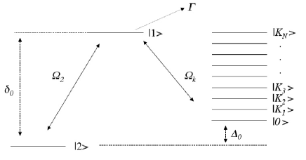
Figure 1: Few-level illustration of free-bound-bound photoassociation. Initially, $N$ atoms are in the Bose-condensed state $|0\rangle$. The free-bound laser then removes two atoms from this state and creates an electronically-excited molecule in the state $|1\rangle$. The bound-bound laser, in turn, removes an excited molecule from the state $|1\rangle$, and creates an electronically-stable molecule in state $|2\rangle$. The quasicontinuum of $N_{qc}$ noncondensate disociation modes is also shown, where a pair of atoms with momentum $\pm\hbar{\bf k}$ and energy $\hbar\epsilon_{k}=\hbar^{2}k^{2}/2m$ are taken to occupy the state $|{\bf K}\rangle\equiv|{\bf k},-{\bf k}\rangle$. The free-bound and bound-bound Rabi frequencies are $\Omega_{k}=\Omega_{1}f_{\bf k}$ and $\Omega_{2}$, where $f_{k}$ denotes the wavevector (energy) dependence of the free-bound coupling. Lastly, the loss rate of the electronically-excited molecular state is $\Gamma$, and the respective intermediate and two-photon detunings are $\delta_{0}$ and $\Delta_{0}$.

Consider a photoassociation laser that removes zero-momentum (${\bf k}=0$) atoms from an initial atomic condensate $|0\rangle$ and creates molecules in the excited molecular condensate $|1\rangle$. A second laser couples this excited molecular condensate with a stable molecular condensate $|2\rangle$. The annihilation operators of the atomic condensate, the excited molecular state and the stable molecular state are denoted by $a_{0}\equiv a$, $b$ and $g$. Transitions to noncondensate atoms arise because a molecule in $|1\rangle$ need not dissociate back to the ${\bf k}=0$ atomic condensate $|0\rangle$, but may just as well wind up as two atoms of equal and opposite momentum ($\pm{\bf k}$) in the state $|{\bf K}\rangle\equiv|{\bf k},-{\bf k}\rangle$, since only relative momentum is conserved. These noncondensate atoms are denoted by $a_{\bf k}$, with $a_{0}\equiv a$ being the condensate. The interactions that cause atom-molecule and molecule-molecule transitions are characterized by their respective Rabi frequencies $\Omega_{\bf k}=\Omega_{1}f_{\bf k}$ and $\Omega_{2}$, where $f_{\bf k}$ expresses the wavevector dependence of the atom-molecule coupling. The one- and two-photon detunings are $\Delta_{0}$ and $\delta=\delta_{0}-i\frac{1}{2}\Gamma$, where the spontaneous decay rate, $\Gamma$, of the excited molecular state is included in the one-photon (intermediate) detuning. This scheme is illustrated in Fig. 1. We also consider s-wave collisions between the atomic and stable-molecular condensates, with interaction strengths $\lambda_{aa}$, $\lambda_{gg}$, and $\lambda_{ag}$. Anticipating large intermediate detunings, the excited-state molecular fraction is low, and its collisions can be ignored; similarly, we also neglect all collisions with noncondensate atoms. Thus, in the rotating wave approximation, the Hamiltonain for the above system is written as

$$\frac{H_{3}}{\hbar} = -\Delta_{0}g^{{\dagger}}g+\delta b^{{\dagger}}b+\sum_{\bf k}\epsilon_{k}a^{{\dagger}}_{\bf k}a_{\bf k}$$ (3)

$$-\frac{1}{2}\sum_{\bf k}\left(\Omega_{1}f_{\bf k}b^{{\dagger}}a_{\bf k}a_{-\bf k}+h.c.\right)-\left(\Omega_{2}g^{{\dagger}}b+h.c.\right)$$

$$+2\lambda_{ag}a^{{\dagger}}ag^{{\dagger}}g+\lambda_{gg}g^{{\dagger}}g^{{\dagger}}gg+\lambda_{aa}a^{{\dagger}}a^{{\dagger}}aa.$$

For simplicity, we take $f_{0}=f^{*}_{0}=1$, $\Omega_{j}=|\Omega_{j}|e^{i\phi_{j}}$, and $f_{\bf k}=f^{*}_{\bf k}$. We also assume free-particles, so that $\epsilon_{k}=\hbar k^{2}/m$, where $m$ is the atomic mass. The atomic condensate modes $a_{0}\equiv a$ are written explicitly in a moment.

We now develop an effective description by adiabatically eliminating the excited molecular state from the Hamiltonian of Eq. (3), based on the Heisenberg equations of motion

$$i\dot{a} = -|\Omega_{1}|e^{i\phi_{1}}a^{{\dagger}}b+2\lambda_{ag}ag^{{\dagger}}g+2\lambda_{aa}a^{{\dagger}}aa,$$ (4)

$$i\dot{a}_{\bf k} = \epsilon_{k}a_{\bf k}-\frac{1}{2}|\Omega_{1}|e^{i\phi_{1}}f_{\bf k}a^{{\dagger}}_{-\bf k}b,$$ (5)

$$i\dot{b} = \delta b-\frac{1}{2}|\Omega_{1}|e^{i\phi_{1}}\sum_{\bf k}f_{\bf k}a_{\bf k}a_{-\bf k}-|\Omega_{2}|e^{-i\phi_{2}}g,$$ (6)

$$i\dot{g} = -\Delta_{0}g-|\Omega_{2}|e^{i\phi_{2}}b+2\lambda_{ag}a^{{\dagger}}ag+2\lambda_{gg}g^{{\dagger}}gg.$$

The trick now is assuming that $\delta$ is the largest frequency in the problem, and we can adiabatically eliminate the excited molecular state by using $\dot{b}/\delta\sim 0$. Thus,

$$b=\frac{|\Omega_{1}|e^{i\phi_{1}}}{2\delta}\sum_{\bf k}f_{\bf k}a_{\bf k}a_{-\bf k}+\frac{|\Omega_{2}|e^{i\phi_{2}}}{\delta}g.$$ (8)

Inserting this into our three-level Hamiltonian of Eq. (3) produces an effectively two-level Hamiltonian. The equations can be simplified by denoting the relative phase of the lasers with $\phi=\phi_{2}-\phi_{1}$, and by writing $\chi=|\Omega_{1}||\Omega_{2}|/\delta$. This yields

$$\frac{H_{2}}{\hbar} = -\Delta^{\prime}g^{{\dagger}}g+\sum_{\bf k}(\frac{1}{2}\Delta_{0}+\epsilon_{k})a^{{\dagger}}_{\bf k}a_{\bf k}$$ (9)

$$-\frac{\chi}{2}\sum_{\bf k}\left(e^{i\phi}g^{{\dagger}}f_{\bf k}a_{\bf k}a_{-\bf k}+{\rm h.c.}\right)$$

$$+2\lambda_{ag}a^{{\dagger}}ag^{{\dagger}}g+\lambda^{\prime}_{aa}a^{{\dagger}}a^{{\dagger}}aa+\lambda_{gg}g^{{\dagger}}g^{{\dagger}}gg,$$

where $\Delta^{\prime}=\Delta_{0}+|\Omega_{2}|^{2}/\delta$ and $\lambda^{\prime}_{aa}=\lambda_{aa}-|\Omega_{1}|^{2}/4\delta$. Note that this is exactly the same form of the Hamiltonian as for one-color transitions, but the two-photon Rabi frequency $\chi$ has replaced the one-photon Rabi frequency $\Omega_{1}$.

Next, we proceed to derive the master equation Meystre & Sargent III (1991); Walls & Milburn (1994) for the stable molecular condensate, applying the same ideas as in Ref. Mackie (2003). Using the interaction picture, the problem is solved to second order in perturbation theory. Taking the atom-molecule condensate as the system, and the noncondensate modes as the environment, the Hamiltonian of Eq. (9) can be written as

$$\frac{H_{2}}{\hbar}=\frac{H_{S}}{\hbar}+\frac{H_{R}}{\hbar}-\left(\frac{\chi}{2}e^{i\phi}g^{{\dagger}}\sum_{{\bf k}\neq 0}f_{\bf k}a_{\bf k}a_{-\bf k}+h.c.\right).$$ (10)

The dynamics is not altered if, for later convenience, we add the constant of motion $\lambda^{\prime}_{aa}(N-N^{2})$ to $H_{2}$ (see also Ref. MAC05b ). Thus, we get $H_{S}=H_{0}+H_{I}$, with

$$\frac{H_{0}}{\hbar} = -\Delta g^{{\dagger}}g,$$ (11)

$$\frac{H_{I}}{\hbar} = -\frac{1}{2}\chi\left(e^{-i\phi}a^{{\dagger}}a^{{\dagger}}g+e^{i\phi}g^{{\dagger}}aa\right)$$ (12)

$$-2\lambda g^{{\dagger}}a^{{\dagger}}ga+(\lambda_{gg}-4\lambda^{\prime}_{aa})g^{{\dagger}}gg^{{\dagger}}g,$$

$$\frac{H_{R}}{\hbar} = \sum_{\bf k\neq 0}\epsilon_{k}a^{{\dagger}}_{\bf k}a_{\bf k},$$ (13)

where $\Delta=\Delta^{\prime}-2\lambda^{\prime}_{aa}+\lambda_{gg}$, and $\lambda=2\lambda^{\prime}_{aa}-\lambda_{ag}$. We then apply the Born approximation and calculate the master equation of our system in the interaction picture. Initially the system $|n_{m}\rangle|n_{a}\rangle$ and the environment $\prod_{\bf k\neq 0}|l_{a}\rangle_{\bf k}$ are not correlated, i.e., $\rho_{tot}=\rho_{s}\otimes\rho_{e}$. The equation of the motion of the total density matrix in the interaction picture is

$$\dot{\rho}_{tot}=-\frac{i}{\hbar}\left[H_{int},\rho_{tot}\right].$$ (14)

After integration, performing the trace over environment and neglecting terms higher than second order, we get

$$\dot{\rho}_{s} = -\frac{i}{\hbar}{\rm Tr}_{e}\left[H_{int}(t),\rho_{s}(0)\otimes\rho_{e}\right]$$ (15)

$$- \frac{1}{\hbar^{2}}\int_{0}^{t}dt_{1}{\rm Tr}_{e}\left[H_{int}(t),\left[H_{int}(t_{1}),\rho_{s}(0)\otimes\rho_{e}\right]\right]$$

$$= \dot{U}_{1}(t)+\dot{U}_{2}(t).$$

In the interaction picture, our Hamiltonian (10) becomes

$$H_{int}=-\hbar\left(A^{{\dagger}}\Gamma+\Gamma^{{\dagger}}A\right),$$ (16)

where we have used the shorthand notation

$$\Gamma = \sum_{{\bf k}\neq 0}f_{\bf k}a_{\bf k}a_{-\bf k}e^{-i(\epsilon_{k}-\Delta)t},$$ (17)

$$A = \frac{\chi}{2}e^{-i\phi}g.$$ (18)

Tracing of Eq. (15) results in

$$\dot{U}_{1}(t)=i\left(\langle\Gamma(t)\rangle\left[A^{{\dagger}},\rho_{s}(0)\right]+\langle\Gamma^{{\dagger}}(t)\rangle\left[A,\rho_{s}(0)\right]\right)$$ (19)

as the first order term, and the second order term is

$$\dot{U}_{2}(t) = -\int_{0}^{t}dt_{1}\left(\langle\Gamma(t)\Gamma(t_{1})\rangle\left[A^{{\dagger}},\left[A^{{\dagger}},\rho_{s}(0)\right]\right]+\langle\Gamma^{{\dagger}}(t)\Gamma(t_{1})\rangle\left[A,\left[A^{{\dagger}},\rho_{s}(0)\right]\right]\right.$$ (20)

$$+ \left.\langle\Gamma(t)\Gamma^{{\dagger}}(t_{1})\rangle\left[A^{{\dagger}},\left[A,\rho_{s}(0)\right]\right]+\langle\Gamma^{{\dagger}}(t)\Gamma^{{\dagger}}(t_{1})\rangle\left[A,\left[A,\rho_{s}(0)\right]\right]\right).$$

The following six coefficients should be calculated:

$$I_{1} = \langle\Gamma(t)\rangle,$$ (21)

$$I_{2} = \langle\Gamma^{{\dagger}}(t)\rangle=I_{1}^{*},$$ (22)

$$I_{3} = \int_{0}^{t}dt_{1}\langle\Gamma(t)\Gamma(t_{1})\rangle,$$ (23)

$$I_{4} = \int_{0}^{t}dt_{1}\langle\Gamma^{{\dagger}}(t)\Gamma^{{\dagger}}(t_{1})\rangle,$$ (24)

$$I_{5} = \int_{0}^{t}dt_{1}\langle\Gamma^{{\dagger}}(t)\Gamma(t_{1})\rangle,$$ (25)

$$I_{6} = \int_{0}^{t}dt_{1}\langle\Gamma(t)\Gamma^{{\dagger}}(t_{1})\rangle.$$ (26)

The coefficients

$$I_{1}=I_{2}=I_{3}=I_{4}=0,$$ (27)

because for the normal thermalized heat bath the correlation function $\langle a_{\bf k}a_{-\bf k}\rangle$ is zero, though these have been studied elsewhere Mackie (2003). In this study, the environment is a thermal cloud around the condensates, and therefore, it is reasonable to assume that it acts like an uncorrelated thermalized heat bath. The nonzero correlations have the form of

$$\langle a_{\bf k}^{{\dagger}}a_{-\bf k}^{{\dagger}}a_{\bf k^{\prime}}a_{-\bf k^{\prime}}\rangle=4\pi n_{k}^{2}\delta_{k,k^{\prime}}.$$ (28)

Let us calculate, say, $I_{5}$:

$$I_{5} = \int_{0}^{t}dt_{1}\langle\Gamma^{{\dagger}}(t)\Gamma(t_{1})\rangle$$ (29)

$$= \int_{0}^{t}dt_{1}\sum_{\bf k}\sum_{\bf k^{\prime}}f_{\bf k}f_{\bf k^{\prime}}4\pi n_{k}^{2}\delta_{k,k^{\prime}}e^{i(\epsilon_{k}-\Delta)t}e^{-i(\epsilon_{k^{\prime}}-\Delta)t_{1}}$$

$$= 4\pi\int_{0}^{t}dt_{1}\sum_{k}f_{k}^{2}n_{k}^{2}e^{i(\epsilon_{k}-\Delta)(t-t_{1})}.$$

The sum can be converted into an integral by assuming that the maximum momentum is very large, i.e., infinite. This approximation will, however, yield consequences that are not present in the original system (maximum momentum very large but finite), e.g., irreversible dynamics. In our case it means that the coherence of the system is decreasing monotonically. Here we have assumed that the particles are in a free space. Of course, if one wants to take the trap into account, one should add here the density of the states of the trap. As the first approximation, we keep the system as simple as possible; neglecting the trap can be justified by the fact that the time scales of the trap are much longer than the assumed decoherence time scale.

Next we go to the frequency representation: $k=\sqrt{m\epsilon/\hbar}$, $d\epsilon=(2\hbar/m)kdk$, so that

$$I_{5}=\frac{m^{3/2}V}{\pi\hbar^{3/2}}\int_{0}^{t}dt_{1}\int_{0}^{\infty}d\epsilon\sqrt{\epsilon}f^{2}(\epsilon)n^{2}(\epsilon)e^{i(\epsilon-\Delta)(t-t_{1})}.$$ (30)

We assume that the Markov approximation is valid, i.e., $\Delta$ is large enough and $\sqrt{\epsilon}f^{2}(\epsilon)n^{2}(\epsilon)$ is a slowly varying function in the vicinity of $\epsilon=\Delta$, and thus the correlation time scale is so short that we can set $t\rightarrow\infty$ in the integral $I_{4}$. These conditions are met when $\hbar\Delta\sim kT$. This leads to the principal value integral

$$\lim_{t\rightarrow\infty}\int_{0}^{t}e^{i(\epsilon-\Delta)(t-t_{1})}=\pi\delta(\epsilon-\Delta)+i\frac{PV}{\Delta-\epsilon}.$$ (31)

Thus,

$$I_{5}=\frac{m^{3/2}V}{\hbar^{3/2}}\sqrt{\Delta}f^{2}(\Delta)n^{2}(\Delta)+i\Delta_{*},$$ (32)

where

$$\Delta_{*}=\frac{Vm^{3/2}}{\pi\hbar^{3/2}}{\rm PV}\int_{0}^{\infty}d\epsilon\frac{\sqrt{\epsilon}}{\epsilon-\Delta}f^{2}(\epsilon)e^{i(\epsilon-\Delta)(t-t_{1})}n^{2}(\epsilon).$$ (33)

While technically related to the Lamb shift, the term $\Delta_{*}$ is the shift that appears anytime one connects a bound state to a continuum. This has been investigated in theory FED96 ; BOH99 and experiment GER01 ; MCK02 ; PRO03 . The shift is neglected in this study. Similarly, for $I_{6}$ we get

$$I_{6}=\frac{m^{3/2}V}{\hbar^{3/2}}\sqrt{\Delta}f^{2}(\Delta)[n(\Delta)+1]^{2}.$$ (34)

The master equation in the interaction picture is thus

$$\dot{\rho}_{int} = -I_{5}\left[A,\left[A^{{\dagger}},\rho\right]\right]-I_{6}\left[A^{{\dagger}},\left[A,\rho\right]\right]$$

$$= (I_{5}+I_{6})(A\rho A^{{\dagger}}+A^{{\dagger}}\rho A-AA^{{\dagger}}\rho-\rho A^{{\dagger}}A).$$

The corresponding master equation in the Schrödinger picture is

$$\dot{\rho}_{s} = -\frac{i}{\hbar}[H_{0}+H_{I},\rho_{s}]+\dot{\rho}_{int}$$ (36)

$$= \frac{i}{\hbar}\left[\Delta(g^{{\dagger}}g\rho-\rho g^{{\dagger}}g)+\frac{1}{2}\chi e^{-i\phi}(a^{{\dagger}}a^{{\dagger}}g\rho-\rho a^{{\dagger}}a^{{\dagger}}g)+\frac{1}{2}\chi e^{i\phi}(g^{{\dagger}}aa\rho-\rho g^{{\dagger}}aa)\right.$$

$$- \left.(\lambda_{gg}-4\lambda^{\prime}_{aa})(g^{{\dagger}}gg^{{\dagger}}g\rho-\rho g^{{\dagger}}gg^{{\dagger}}g)+2\lambda(g^{{\dagger}}a^{{\dagger}}ga\rho-\rho g^{{\dagger}}a^{{\dagger}}ga)\right]$$

$$+ (I_{5}+I_{6})(A\rho A^{{\dagger}}+A^{{\dagger}}\rho A-AA^{{\dagger}}\rho-\rho A^{{\dagger}}A),$$

where $H_{I}$ is treated as a perturbation.

III Simulations

The aim of the present work is to study the impact of the rogue decoherence environment. It is important to note that it is a matter of contention whether strong two-color photoassociation of a Bose-Einstein condensate is even possible MAC05 . We insist that it is and, moreover, that it is possible to target ground-electronic state levels that are sufficiently low-lying to allow neglect of vibrational-relaxation losses (see also MAC05b ) Our simulations therefore consist of two stages: first, a particular joint-atom molecule condensate with real probability amplitude is created in the regime where photoassociation is much stronger than collisions; second, the photoassociation intensity is reduced and the joint atom-molecule condensate evolves under now-dominant collisional interaction into a macroscopic atom-molecule superposition.

Emipircally Calsamiglia, Mackie & Suominen (2001), we have found that the parameter values that are sufficient to create the proper Phase-$I$ joint atom-molecule condensate are:

$$\Delta = 0,$$ (37)

$$\chi = 10\sqrt{N}\lambda,$$ (38)

$$\phi = \pi/2.$$ (39)

By proper, we mean a joint atom-molecule condensate with a real amplitude Calsamiglia, Mackie & Suominen (2001), which is the origin of the relative phase $\phi=\pi/2$, and where half the original atoms have been converted to molecules. The duration of the strong two-photon-resonant photoassociation pulse is $\tau$, which can be obtained from the solution of the semiclassical approximation for the molecules Calsamiglia, Mackie & Suominen (2001), $N/4=(N/2)\tanh^{2}(\sqrt{N}\chi\tau)$, which is a result borrowed from the theory of second-harmonic-generated photons Walls et Tindle (1972). The condition $\Delta=0$ means that the system is on a Stark-shifted resonance and the Markov approximation becomes dubious. On resonance, the interaction strength compared to the evolution time scale increases and one expects that decoherence would take a more dominant role. Thus, we use a large enough two-photon detuning, $\Delta>kT$, to avoid the resonance and justify the Markov approximation: $\Delta=0.1N\lambda$, for $\rho=1.88\times 10^{19}{\rm m^{-3}}$.

The second phase is collision-dominant:

$$\Delta = \sqrt{N}\chi=0.1N\lambda,$$ (40)

$$\chi = 0.1\sqrt{N}\lambda,$$ (41)

$$\phi = 0.$$ (42)

The collision interactions are

$$\lambda_{aa} = \frac{4\pi\hbar a_{aa}}{mV},$$ (43)

$$\lambda_{ag} = \frac{3\pi\hbar a_{ag}}{mV},$$ (44)

$$\lambda_{gg} = \frac{2\pi\hbar a_{gg}}{mV},$$ (45)

where the atom-atom scattering length is $a_{aa}=5.4$ nm Drummond et al. (2002); Wynar et al. (2000), the atom-molecule scattering length is $a_{ag}=-9.346$ nm Drummond et al. (2002); Wynar et al. (2000), the unknown molecule-molecule scattering length is approximated as $a_{gg}=a_{aa}$, the mass of a ${}^{87}{\rm Rb}$ atom is $m=1.443\times 10^{-25}$ kg, and $V$ is the quantization volume that is expedient in a partiuclar context (e.g., cubic box, spherical cavity, or harmonic trap). Also, by optically tuning the atom-atom scattering length FED96 ; BOH97 ; BOH99 ; FAT00 ; THE04 ; THA05 , there is the possibility to reduce the number of parameters by setting $\lambda_{gg}-4\lambda^{\prime}_{aa}=0$, which amounts to $a_{aa}^{\prime}=a_{gg}/8$. The effects of the loss term $\Gamma=12\times 2\pi~{}{\rm MHz}$ Wynar et al. (2000) should be negligible if $|\delta|>>\Gamma$; therefore, we choose $|\delta|\sim 10^{3}\times 2\pi~{}{\rm MHz}$. For this detuning, and barring an anomalously large molecule-molecule scattering length, the light-induced scattering-length shift should be possible; however, this really only a matter of convenience, and is not neccesary. Finally, with the given value of $\lambda^{\prime}_{aa}$, the remaining collisional interaction strength is $\lambda=(\rho/N)\times 7.67715\times 10^{-17}\,{\rm Hz}$, where $[\rho]\equiv m^{-3}$.

We use the molecular number basis: $\rho=|m\rangle\langle m^{\prime}|$, where $m$ and $m^{\prime}$ are the molecule numbers, and $N$ is the total particle number. Hence, the coupled equations to solve are

$$\begin{array}[]{cclcl}\dot{\rho}_{m,m^{\prime}}&=&\rho_{m,m^{\prime}}\{i\Delta(m-m^{\prime})+i2\lambda[(N-2m)m-(N-2m^{\prime})m^{\prime}]&-&(I_{5}+I_{6})\frac{\chi^{2}}{4}m^{\prime}\}\\ &-&\rho_{m,m^{\prime}}(I_{5}+I_{6})\frac{\chi^{2}}{4}(m+1)&;&m<N/2\\ &+&\rho_{m-1,m^{\prime}}i\frac{1}{2}\chi e^{-i\phi}\sqrt{(N-2m+1)(N-2m+2)m}&;&m>0\\ &-&\rho_{m,m^{\prime}+1}i\frac{1}{2}\chi e^{-i\phi}\sqrt{(N-2m^{\prime})(N-2m^{\prime}-1)(m^{\prime}+1)}&;&m^{\prime}<N/2\\ &+&\rho_{m+1,m^{\prime}}i\frac{1}{2}\chi e^{i\phi}\sqrt{(N-2m)(N-2m-1)(m+1)}&;&m<N/2\\ &-&\rho_{m,m^{\prime}-1}i\frac{1}{2}\chi e^{i\phi}\sqrt{(N-2m^{\prime}+1)(N-2m^{\prime}+2)m^{\prime}}&;&m^{\prime}>0\\ &+&\rho_{m-1,m^{\prime}-1}(I_{5}+I_{6})\frac{\chi^{2}}{4}\sqrt{mm^{\prime}}&;&m,m^{\prime}>0\\ &+&\rho_{m+1,m^{\prime}+1}(I_{5}+I_{6})\frac{\chi^{2}}{4}\sqrt{(m+1)(m^{\prime}+1)}&;&m,m^{\prime}<N/2.\end{array}$$ (46)

Let us stress that these equations of motion (46) behave well at the thermodynamical limit $V\rightarrow\infty$ because, as typical for photoassociation, $\chi\sim 1/\sqrt{V}$ Javanainen et Mackie (1999); Kostrun et al. (2000), $I_{5}+I_{6}\sim V$ and $\rho_{m,m^{\prime}}\sim 1/N$.

The common decay profile of coherence in infinite models has the form of $e^{-t/\tau_{d}}$, which defines the decoherence time $\tau_{d}$ Unruh et Zurek (1989); Zurek (1991). Phase $I$ follows this usual behavior, and has the off-diagonal decoherence time

$$\tau_{d,{\rm off}}=\frac{4}{\chi^{2}(I_{5}+I_{6})}=\frac{4\hbar^{3/2}\rho}{m^{3/2}\chi^{2}\sqrt{\Delta}N(2n^{2}+2n+1)},$$ (47)

where the total particle number is $N$ and the fraction of noncondensate atoms is $n=1/[\exp(\hbar\Delta/kT)-1]$. Since photoassociation is dominant by design, this timescale must be compared to the photoassociation time scale $\tau_{pa}=(\sqrt{N}\chi)^{-1}$. The decoherence condition is thus

$$\xi_{d,I}=\frac{\tau_{d}}{\tau_{pa}}=\frac{2.712057\times 10^{10}}{\sqrt{\rho[{\rm m^{3}}]}(2n^{2}+2n+1)},$$ (48)

where we have used the detuning $\Delta=0.1N\lambda$. In most simulations we have used a small but realistic temperature $T=10^{-9}{\rm K}$. Thus, the validity of the Markov approximation requires $\Delta>131{\rm Hz}$. The nonzero detuning, compared with zero detuning, in the phase $I$ does not contribute much to the moment $\tau$ when phase $I$ ends. The generalized Rabi frequency Harter et al. (1981) is $\chi_{gen}=\sqrt{N\chi^{2}+\Delta^{2}}=N\lambda\sqrt{100+0.01}$. For simplicity, we do not apply the time boundary between phases $I$ and $II$ given by the semiclassical approximation [i.e., $\tau$ defined by $N/4=(N/2)\tanh^{2}(\sqrt{N}\chi\tau)$], but we instead optimize the distance between the two superposition peaks, or, the “size” of the superposition, to be a large as possible. An optimal superposition size, and equally-sized probability peaks, are obtained only if the phase $I$ ends at the moment $\tau$ when ${\rm Tr}\rho g^{{\dagger}}g\sim 0.296N/2$. This end point is very sensitive: the accuracy in molecular fraction should be $\sim\pm 0.001$ in order to get equally sized peaks. Also, the end point depends a bit on the particle number. The above mentioned result is valid for $N=1000$.

Phase $II$ follows similar behavior, having the same decoherence time as in Eq. (47). However, since collisions are dominant in phase $II$, we compare the decoherence time in phase $II$ with the collision time scale $\tau_{c}\sim(2N\lambda)^{-1}$. Hence, the decoherence condition is

$$\xi_{d,II}=\frac{\tau_{d}}{\tau_{c}}=\frac{2.408246\times 10^{10}}{\sqrt{\rho[{\rm m^{3}}]}(2n^{2}+2n+1)}.$$ (49)

If phase $I$ results in suitable initial conditions to produce a macroscopic superposition in phase $II$, decoherence in phase $II$ is the only remaining thing to prevent the superposition state. The correlations created by collisions are the mechanism that, in ideal conditions, results in a macroscopic superposition of atomic and molecular condensates. Therefore, if the decoherence time scale is smaller than the collisional time scale then decoherence dominates over collisions and prohibits the creation of the macroscopic superposition. The constraint to the superposition here is $\xi_{d,II}>>1$.

There are several damping scenerios to consider; although, due to limited computational resources, we consider the case of $N=1000$ particles. In scenario $A$ there is no decoherence present, i.e., $\xi_{d,I}=\xi_{d,II}\approx\infty$. In scenerio $B$, the parameter values $\rho=1.88\times 10^{19}~{}{\rm m^{-3}}$ and $T=10^{-9}~{}{\rm K}$ result in moderate decoherence, i.e., $\xi_{d,I}=3.44$ and $\xi_{d,II}=3.05$. The scenario $C$ is the borderline scenario with $\xi_{d,I}=\xi_{d,II}=1$. Corresponding temperatures and densities can be calculated from Eqs. (48) and (49). In scenario $D$, we assume a temperature $T=10^{-10}~{}{\rm K}$ and density $\rho=1.88\times 10^{18}{\rm m^{-3}}$, i.e., $\xi_{d,I}=10.88$ and $\xi_{d,II}=9.65$. The results are illustrated in Figs. 2-4. In Fig. 2 we present the probability distributions of all scenarios at two different instants of time. The first instant ($t_{1}$) is when the phase $I$ ends, and a particular joint-atom molecule condensate with a real probability amplitude is created. It serves most ideal initial conditions to begin the collision dominant phase $II$. The second instant ($t_{2}$) is when the superposition peaks should emerge. Figure 3 presents the density matrices of all scenarios at $t_{1}$, and Fig. 4 the density matrices of all scenarios at $t_{2}$.

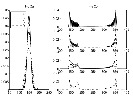
Figure 2: The probability distributions of scenarios $A$ (no damping), $B$ (moderate damping), $C$ (strong damping) and $D$ (weak damping) at (a) $\lambda t_{1}=8.6\times 10^{-5}$ when the stage $I$ ends and (b) at $\lambda t_{2}=1.0486\times 10^{-2}$ when the superposition state emerges at the end of stage $II$. Decoherence obviously affects the probability distributions: stronger decoherence makes the probability peaks lower and wider. Recall that the stage $I$ and $II$ decoherence conditions for the various scenerios are ($A$) $\xi_{d,I}=\xi_{d,II}\approx\infty$; ($B$) $\xi_{d,I}=3.44$ and $\xi_{d,II}=3.05$; ($C$) $\xi_{d,I}=\xi_{d,II}=1$; and, ($D$)$\xi_{d,I}=10.88$ and $\xi_{d,II}=9.65$.

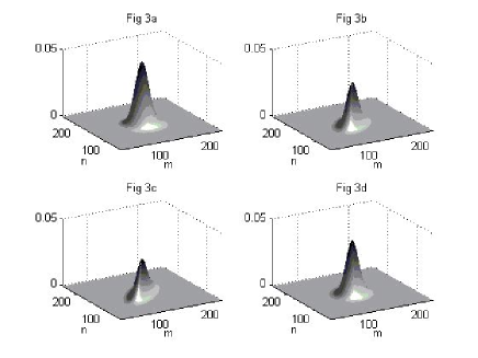
Figure 3: The density matrices of scenarios $A$ (a, no damping), $B$ (b, moderate damping), $C$ (c, strong damping) and $D$ (d, weak damping) at the end of stage $I$ at $t_{1}$. Decoherence effects are clearly visible in scenarios $B$ and $C$, as the decay of off-diagonal elements has resulted in ellipsoid-gaussian wave packet. Again, recall the decoherence conditions: $A$, $\xi_{d,I}=\xi_{d,II}\sim\infty$; $B$, $\xi_{d,I}=3.44$ and $\xi_{d,II}=3.05$; $C$ $\xi_{d,I}=\xi_{d,II}=1$; and $D$, $\xi_{d,I}=10.88$ and $\xi_{d,II}=9.65$.

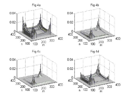
Figure 4: The density matrices of scenarios $A$ (a, no damping), $B$ (b, moderate damping), $C$ (c, strong damping) and $D$ (d, weak damping) at $t_{2}$, when a macroscopic superposition state should emerge. Only a small fraction of off-diagonal elements have survived from decoherence, even in the scenario $D$, that has extreme parameter values of $T=10^{-10}{\rm K}$ and $\rho=10^{18}{\rm m^{-3}}$. Again, recall the decoherence conditions: $A$, $\xi_{d,I}=\xi_{d,II}\sim\infty$; $B$, $\xi_{d,I}=3.44$ and $\xi_{d,II}=3.05$; $C$ $\xi_{d,I}=\xi_{d,II}=1$; and $D$, $\xi_{d,I}=10.88$ and $\xi_{d,II}=9.65$.

Overall, while decoherence is strong enough, the quantum correlations are damped out and sharp peaks in probability distributions smoothen. The decay of off-diagonal elements seems to be considerable also in the regime of moderate decoherence $1<\xi_{d}<6$. Strong decoherence effects $\xi_{d}<1$ would be even faster. In order to get a macroscopic superposition with the given setup, one should be safely in the regime of weak decoherence, i.e., $\xi_{d}>10$. However, the regime is not reachable using parameter values consistent with present-day technology. Of course, there are a few possibilities to improve the result and get $\xi_{d}>10$. First, one can reduce the density $\rho$, but $10^{19}{\rm m^{-3}}$ is somewhat rarified as it is, even for a condensate, and achieving $2\times 10^{18}{\rm m^{-3}}$ could present challenges. The second possibility is to enter the non-Markovian regime, which could considerably improve the $\xi_{d}$ at least in phase $I$; however, the non-Markovian case will be studied elsewhere. Other tricks are related to manipulating the interaction or the environment. The symmetrization of the environment Dalvit, Dziarmaga, and Zurek (2000) would be a hard, maybe impossible, task to apply here due to the inherent nonlinearity; but, creating specially a correlated environment might help since an uncorrelated heat bath is quite a harsh environment for coherence phenomena.

Finally, we note that the observation of the possible superposition state could present a problem. The assumption that the coherence of the state after phase $I$ can be verified, and thus one only needs to consider the density matrix profiles of the revival of this initial state after the superposition state Calsamiglia, Mackie & Suominen (2001); Huang et Moore (2005), is perhaps too simple, at least in the Markovian regime. While the system is driven from superposition to the revived state, rogue dissociation is still damping coherence out of the system. Also, coherent tricks, such as phase-imprinting the revived state, would need extra time, and this introduces more decoherence. The best candidate for observing the macroscopic superposition is probably to try to entangle the superposition state with another system, and then to apply Bell-type correlation experiments.

IV Discussion

The important point is that our approach is a dynamical one in which we make the macroscopic superposition in the presence of the decoherence, which differs from the standard way in which one takes the macroscopic superposition for granted and then puts it into a decoherent environment and looks how long it would last there. Such studies do not make claims whether it is possible to create a macroscopic superposition or not, but they only make claims whether the initially prepared macroscopic superposition can be observed or not. Therefore, our photoassociation-based approach suggests a possible experimental creation of the macroscopic superposition in a decohering environment.

Hence, the aim of this study is to understand the effects of the rogue-dissociation-induced decoherence while trying to create a macroscopic superposition of Bose-condensed atoms and molecules. In particular, ours is a two-stage scheme: in the first stage, the photoassociation coupling is strong compared to the s-wave collisional coupling, and a specific joint atom-molecule condensate is created; in the second stage, the photoassociation coupling is turned down such that it is weak compared to the collisional coupling, and the system evolves into a macroscopic atom-molecule superposition. There is a constraint $\xi_{d}>>1$, which should be satisfied in order to get a macroscopic superposition of atoms and molecules. The dependency on relevant system parameters of the constraint $\xi_{d}$ was calculated in both stages of our theoretical setup. An interesting fact is that, for the given parameter ratios, $\xi_{d}$ does not depend on the number of particles in condensate $N$. Results for a modest, say, $N=1000$ particle superposition state will therefore apply to a $N=10^{9}$ particle superposition state with the same density, given properly scaled laser frequencies and intensities. Using $\xi_{d}$ one can easily, without heavy simulations, consider whether the macroscopic superposition state of atoms and molecules is within reach or not with given experimental setup parameters.

Without any tricks, the best chance to defeat rogue decoherence in creating an atom-molecule superposition corresponds to a density $\rho=2\times 10^{18}~{}{\rm m^{-3}}$ and temperature $T\sim 0.1~{}{\rm nK}$. Nevethless, while this temperature may be accessible by making the trap shallow, the off-diagonal elements of density matrix will still experience considerable decay. One way to get better macroscopic superpositions in the present scheme is to challenge the assumptions or approximations of our study or, in other words, engineer the environment. We assumed that the environment is an uncorrelated heat bath, the system parameter values should be in the regime where Markov approximation is valid, the environment particles are free and the environment is infinite. Indeed, it may well prove interesting to examine the non-Markovian regime, where a greater part of the physically-relevant parameter space is available, and/or to use a specially correlated environment.

Rogue dissociation is an important source of decoherence that should not be neglected in coherence studies of atom-molecule Bose-Einstein condensates. Unfortunately, it seems to push coherent atom-molecule engineering (macroscopic superpositions, quantum computation, etc.) one step further away from realization.