Trend arbitrage, bid-ask spread and
market dynamics

Abstract

Microstructure of market dynamics is studied through analysis of tick price data. Linear trend is introduced as a tool for such analysis. Trend arbitrage inequality is developed and tested. The inequality sets limiting relationship between trend, bid-ask spread, market reaction and average update frequency of price information. Average time of market reaction is measured from market data. This parameter is interpreted as a constant value of the stock exchange and is attributed to the latency of exchange reaction to actions of traders. This latency and cost of trade are shown to be the main limit of bid-ask spread. Data analysis also suggests some relationships between trend, bid-ask spread and average frequency of price update process.

1 Introduction

Question about market microdynamics is of fundamental importance. It influences wide range of items: bid-ask spread dynamics, interaction of market agents setting market and limit orders, patterns of price formation and provision of liquidity. These subjects are investigated using wide range of analytic tools, trying to capture cross-correlation structure of price evolution and volatilities through time series analysis [Roll] or studying dynamics of price formation through simulation of detailed market mechanics [Smith et.al.] . These methods concentrate on search of the source of random forces acting over continuous or discrete time sets. These sets are considered homogeneous when long-term returns are considered. On the shorter scale (in tick data), it is noticed that the trading frequency scales the returns making time sets non-homogeneous. Theoretical construction is built in [Derman] to account for such effect.

In contrast to statistical methods, the behavioral finance searches patterns of dynamics of collective actions of various market agents making assumptions about their perception and searching for equilibrium and/or limiting solution to price/spread prediction problem [Schleifer, Bondarenko].

All above mentioned methods analyze price returns. In this article we introduce new object for such analysis, a trend . Common definition of trend is ”the general direction in which something tends to move”. Visually trend can be identified as a line with little random deviations. Of course, trends were studied many times before. However, they were studied often in relation to question of deterministic behavior of price.

We think, that the existence of trend is not $necessarily$ deterministic and in general does not disapprove statistical nature of price behavior. Indeed, there is a non-zero probability to find straight line in price path generated using, for example, Black-Scholes model [Durlauf]. Despite this fact, crowd of market participants still believes that such trends are due to some hidden bits of information and therefore contribute to trend persistence or otherwise.

In this paper we would like to merge these two ideas of considering price evolution through scope of trend and through random walk. Indeed, the presentation of price path in terms of price returns (random walk) is suitable in connection to CAPM and alike theories, where profit and risks are related in search of optimal investment portfolio. On the other side, presentation of price evolution in terms of short-term price trends better conforms description of market microdynamics.

The trend is an object worth to study because as we show it gives insight into microstructure of market dynamics. It allows direct observation of spread dynamics, price information update, costs, trading activity and response time of the exchange. This information is diluted when correlation analysis of price return series is used. In this paper trends are studied without consideration of news impact to the price move but only in relation to dynamics of agents interaction via exchange.

Exchange is a dynamic system. It allows traders to interact with each other. It consists of many components. These parts are specialists on the floor, electronic platform which helps to account and match trades through software and a wire connection to trader computers. Traders use electronic platforms to trade. Both systems, of traders and of exchange, have their respective non-zero latencies and therefore the speed of information diffusion is non-zero . The latencies influence price dynamics and respective trading algorithms.

This study draws attention to the influence of dynamics of systems used for trading on the dynamics of price. We extract information content of such dynamics from trends and spreads data.

The article is organized as follows. First, we discuss trend arbitrage. The respective relationship has been derived and is taken as starting point to further analysis. Second, one applies an algorithm searching for linear trend in time series of bids and asks observed on stock markets. Third, several distributions are obtained to support the relationship developed from trend arbitrage requirement. Several outcomes have been discussed as well.

2 Trend Arbitrage

In the following, one analyze intra-day trend seen in prices of an asset which is traded in double auction.

For brevity of explanation we assume two kind of market agents: Specialists and Investors. Specialists maintain sell- and buy-prices (asks and bids, respectively) in continuous manner. Bids and asks generally move together. Spread between them (spread=ask-bid) tends to some minimum level due to competition between Specialists. This level depends on risk perceived by Specialists to take their market share. In stress situations, especially when price directionally moves to the new level, spread increases. The question now is what this dependency is.

A simple example helps to find an answer. Specialist provides bid and ask prices earning spread. Investor profits by taking directional bets. Suppose now that the price moves within up-trend, $\mu$, with spread, $Spr$, see Figure 2.

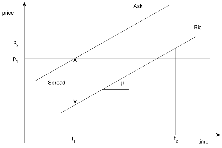
Figure 2: Trend arbitrage relationship.

Investor buys asset at ask-price, $p_{1}$, at $t_{1}$ moment. After a while he sells it. If the trend did not change its direction and Investor waits long enough, till time $t_{2}$, he can sell asset at bid-price, $p_{2}$. Investor will make no profit if:

$$0\geq p_{2}-p_{1}-Spr+\mu\cdot(t_{2}-t_{1})$$ (1)

Investor must meet three conditions to profit for sure:

• $|\mu|$ is non decreasing during the period between $t_{1}$ and $t_{2}$;

• trading system of Investor is faster than that of Specialist and trading system of Specialist is slower than some market reaction value, $\tau$;

• spread is small enough, satisfying (1).

Knowing these conditions (consciously or not), Specialist sets spread such that he makes no losses, i.e. $p_{2}$ is kept equal to $p_{1}$ or less.

Same arguments are applied to down-trend, which changes $\mu$ to $|\mu|$. Therefore, (1) is modified and limit on spread can be set:

$$Spr\geq|\mu|\cdot\tau$$ (2)

where $\tau=t_{2}-t_{1}$. More general expression must also include additional costs to be paid by Investor related to his trading activity and some structure of characteristic time, $\tau$:

$$Spr\geq|\mu|\cdot(\tau_{M}+\tau_{S})+fee$$ (3)

where $fee$ is a broker fee and similar additive costs, $\tau_{M}$ is exchange-wide latency and $\tau_{S}$ is stock specific latency. $\tau_{S}$ can be attributed to aggregated latencies of trading platforms used by Investors to trade the same stock.

These inequalities suggest that the non-zero spread is due to both, transaction costs and latencies of trading and exchange systems.

Now, let us look at the relationships through data analysis perspective.

3 Data analysis

3.1 Data

Tick price/volume data of 33 stocks traded at Amsterdam (NLD), Frankfurt (GER), Madrid (SPA), Paris (FRA) and Milan (ITL) were collected over the second half of the year 2003. This data includes bid, ask and trade prices and respective volumes attached to time stamps. Time period considered is between 15:30 and 17:30 of European time . Dividend information was not used because it does not affect our intraday analysis.

Data were filtered. Only those bits of information were used in analysis where price of either bid or ask has been updated. Any such change is treated as ”information update”.

3.2 Trend identification

Linear fit (details can be found elsewhere [Wiki]) was applied to series of one day mid-prices, $(ask(t_{i})+bid(t_{i}))/2$. Bid-ask spread, $\epsilon(t_{i})=(ask(t_{i})-bid(t_{i}))$, is understood as an uncertainty of observed price information (this item to be discussed further). Data were fit continuously. This way real-time feed is simulated, where only past information is available. An output of fit is series of current trend parameters such as series of impact, $p_{0}(t_{i})$, series of slope (trend), $\mu(t_{i})$, with respective errors, $\epsilon_{p}(ti)$, $\epsilon_{\mu}(ti)$. These parameters allow prediction of forward price, $\tilde{p}$, and price error, $\epsilon$:

$$\tilde{p}(t_{i})=p(p_{0}(t_{i-1}),\mu(t_{i-1}),t_{i})\textrm{, and}$$ (4)

$$\tilde{\epsilon}(t_{i})=\epsilon(p_{0}(t_{i-1}),\mu(t_{i-1}),\epsilon_{p}(t_{i-1}),\epsilon_{\mu}(t_{i-1}),t_{i}).$$ (5)

Condition to trigger end of current trend:

$$\frac{|\tilde{p}(t_{i})-p(t_{i})|}{\sqrt{\tilde{\epsilon(t_{i})}^{2}+\epsilon(t_{i})^{2}}}>n$$ (6)

where $n$ is cut value, which is chosen to be equal to 2.3. This particular choice of cut-off value was determined visually from trends superimposed on the price plot (see Figure (4). There is an intuitive feeling that the less cut-off value generates too many spurious trends and dilutes effects we are looking for. Use of price returns is a limiting case for trends with just two points. On the other side, the larger cut-off value will lead to reduced sensitivity of spread information to trends.

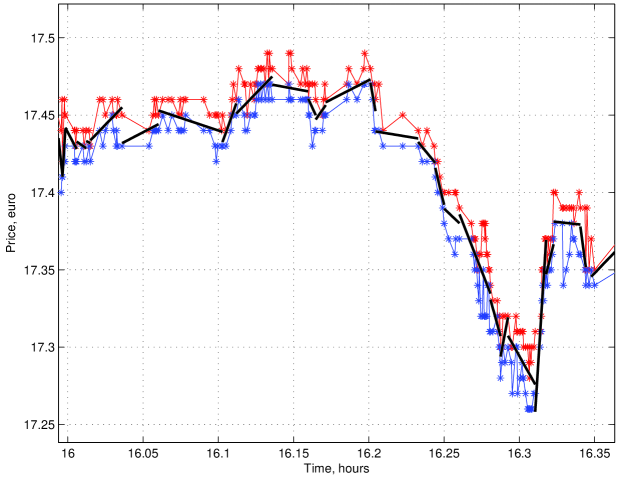
Figure 4: Trend fit to bid-ask series of ABN-AMRO. Star-points connected with lines are bid and ask prices (in blue and red, respectively), piece-wise solid lines in between are fitted trends.

Trend search starts at the beginning of each day series with a seed of three points. Algorithm continues to fit line till the trigger (6) is hit. It then assumes that within the search time window (between current point and the beginning of current trend) there are two trends. Algorithm starts backward search in order to find an optimal breaking time point between current and forward trends. The point is found at the minimum of $\chi^{2}_{t}=(\chi^{2}_{t})_{cur}+(\chi^{2}_{t})_{fwd}$, where $(\chi^{2}_{t})_{i}$ are of current ($i=cur$) and of forward ($i=fwd$) trends. This point becomes the end of current trend and the start of forward one. The forward trend becomes current. And so on till the end of day. Each trend is then accompanied with respective information:

• start and end point within time series, $t_{0}$ and $t_{e}$;

• duration of trend in seconds, $\Delta T=t_{e}-t_{0}$;

• slope, $\mu$, impact, $p_{0}$, and respective errors, $\epsilon_{s}$, $\epsilon_{p}$ found at end-point, $t_{e}$;

• quadratic average spread, $\tilde{Spr}=\sqrt{\frac{\Sigma\epsilon^{2}}{n}}$;

• number of data points in the fit, $N_{u}$. $\tau_{u}=\Delta T/N_{u}$ average time between updates of price (bid or ask) information. $\tau_{u}$ is also called average update time;

• $\chi^{2}_{t}$ of the fit, where

  $$\chi^{2}_{t}=\sum_{i}\frac{(\tilde{p}(t_{i})-p(t_{i}))^{2}}{(\epsilon_{p})_{i}^{2}}$$

  
  

  Trends and associated data found from intraday data were merged into one single dataset day-by-day. For further analysis a selection cut was applied to filter badly fit trends:

  • $\chi^{2}_{t}$-probability, $Prob(\chi^{2}_{t},n.d.f.)<0.99$, where $n.d.f=N_{u}-2$;

  • number of points in the fit $>4$;

  3.3 Price uncertainty

  Trend measurement rises important question: what is the measurement error of observed price? One possibility is to interpret mid-prices as observed exactly with equal weights. The errors of fitted line parameters can be estimated from the sample in a standard way. Another way is to assume that the price is governed by some diffusion process and therefore to interpret estimated volatility as current price errors. Both methods seem not acceptable since they do not bear instant information about price uncertainty.

  We believe that the bid-ask spread is a good candidate to estimate instant price uncertainty. In principle, the price error (and spread) must be dependent on the volume to be traded by some arbitrage algorithm, which uses the trend fit. In this case all analysis will change. In this research we concentrate on analysis of the best bids-asks dynamics alone.

  Example of distribution of $\chi^{2}_{t}$-probability (see Figure 6) demonstrates that our choice is overall correct because the probability is mostly flattened in range [0,1]  peaking at 1.

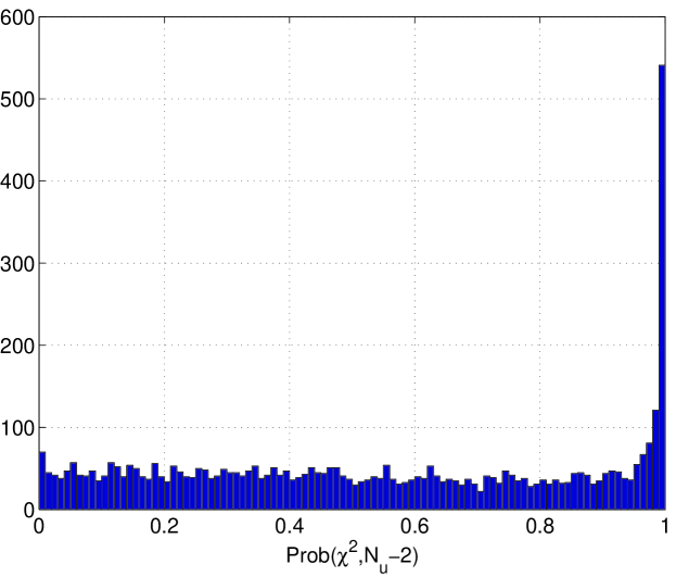
Figure 6: $\chi^{2}$ probability for all found ABN-AMRO trends.

The rejected trends with $\chi^{2}_{t}>0.99$ tend to have smaller $|\mu|$. In case of less expressed trends the market enters intermediate regime known from technical analysis as ”side trend”.

4 Results

4.1 Test of trend arbitrage

4.1.1 Market reaction time, $\tau_{M}$

Let us make trivial rearrangement of Equation (3) by moving observables to the left side of inequality and dividing both sides by $\mu$:

$$\frac{Spr}{|\mu|}-\tau_{S}\geq\tau_{M}+\frac{fee}{|\mu|}$$ (7)

To test this expression we measure $Spr$ as $\tilde{Spr}$, the average update time, $\tau_{S}$, as $\tau_{u}$ and $\mu$ as trend slope (all are defined in previous section (sec. 3.2)). A distribution of $\tau_{resp}=\frac{\tilde{Spr}_{i}}{|\mu_{i}|}-(\tau_{u})_{i}$ value for all $i$-trends found in ABN-AMRO stock price, is plotted on Figure 8. Comparison of ABN-AMRO quantiles of $\log{\tau_{resp}}$ with quantiles of normal distribution and with quantiles of $\log{\tau_{resp}}$ for several other stocks indicate their similarity to log-normal p.d.f. and between each other, see Figure 10.

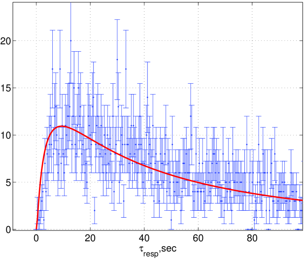
Figure 8: Distribution of $\tau_{resp}$ for ABN-AMRO stock. Red line indicates log-normal fit.

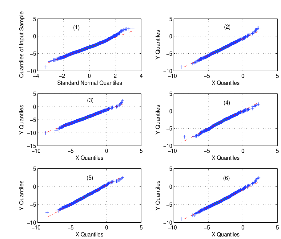
Figure 10: Quantiles of $\log{\tau_{resp}}$ of ABN-AMRO compared with quantiles of Normal distribution (1) and with quantiles of $\log{\tau_{resp}}$ of AEGON/NL (2), Daimler-Crysler/GE (3), BBVA/SP (4), Repsol YPF/SP (5) and AXA/FR (6).

$\tau_{resp}$-distribution starts sharply at some moment after ’zero’-time which is market reaction time, $\tau_{M}$ (see (7)), assuming $\frac{fee}{\mu}$ equal to zero. $\tau_{M}$ value is calibrated using $max(0,f(x))$, where $f(x)$ is log-normal function. The front-end value is calculated at 1% of fitted log-normal p.d.f.. $\tau_{M}$ values per stock are plotted in Figure 12. Exchange averages of $\tau_{M}$, $\tilde{\tau_{M}}$, are given on the same plot and are quoted in Table 2.

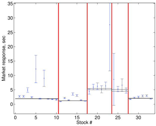
Figure 12: $\tau_{M}$ values measured per stock (numbered from 1 to 33). Results are sorted by exchanges where stocks are traded in bands separated by vertical lines. Exchanges (left to right) are Amsterdam (NLD), Frankfurt (GER), Madrid (SPA), Milano (ITL) and Paris (FRA). Horizontal lines indicate range of $\tau_{M}$ for each exchange.

Table 2: Exchange averages of measured $\tau_{M}$.

Exchange	$\tilde{\tau_{M}}$
Amsterdam (NLD)	1.9 $\pm$ 0.1
Frankfurt (GER)	1.22 $\pm$ 0.04
Madrid (SPA)	5.5 $\pm$ 0.5
Milano (ITA)	5.1 $\pm$ 0.6
Paris (FRA)	2.1 $\pm$ 0.1

$\tau_{M}$ values are grouped clearly by respective exchanges, which suggest universality of this parameter within every particular market. In principle, the inequality (7) does not force all Specialists to set prices close to the very limit, $\tau_{M}+\frac{fee}{|\mu|}$. Competition does, however.

4.1.2 Structure of $\tau_{resp}$: $fee$ and again $\tau_{M}$

Inequality (7) defines linear edge $\tau_{M}+\frac{fee}{|\mu|}$ for 2D-distribution $(\tau_{resp};\frac{1}{|\mu|})$. Figure 14 supports this idea in general. However, zooming into the picture, see Figure 16, suggests some structure which probably reflects the investment horizon of Investors: fast (short/intraday horizon), medium and slow (long horizon).

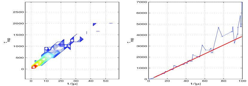
Figure 14: Left plot: 2D-distribution of $\tau_{resp}$ (Y-axis) and $1/|\mu|$ (X-axis) for ABN-AMRO. Solid line indicates edge. Right plot: Edge values of $\tau_{resp}$ obtained from vertical slices of 2D-plot on the left.

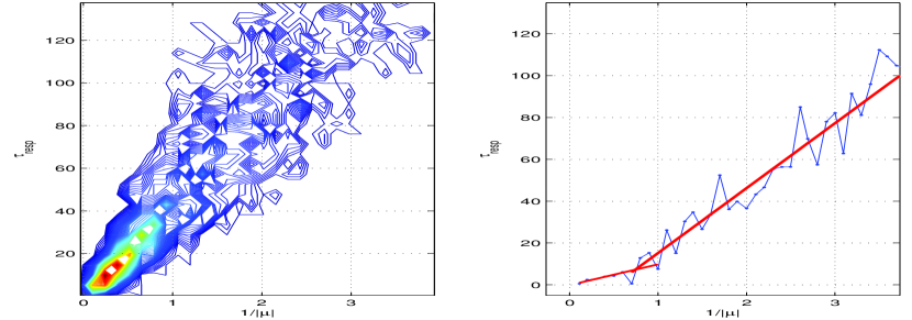
Figure 16: Zoom of Figure 14. Left-plot: 2D-distribution of $\tau_{resp}$ (Y-axis) and $1/|\mu|$ (X-axis) for ABN-AMRO. Solid line indicates edge. Right plot: Edge values of $\tau_{resp}$ obtained from vertical slices of 2D-plot on the left.

Measurement of $fee$ and $\tau_{M}$ parameters for all three groups for all stocks are given in the Table 4.

Table 4: $\tau_{M}$ and $fee$ measured from $(\tau_{resp},\frac{1}{\mu})$ 2D-distribution.

Market	Stock	$fee\pm\epsilon_{fee}$			$\tau_{M}\pm\epsilon_{\tau_{M}}$
	No.	fast	medium	slow	fast	medium	slow
NLD	1	10 $\pm$ 2	30 $\pm$ 6	38 $\pm$ 2	-0.1 $\pm$ 0.3	-14 $\pm$ 11	-62 $\pm$ 187
	2	14 $\pm$ 3	32 $\pm$ 5	37 $\pm$ 1	-1.5 $\pm$ 0.4	-17 $\pm$ 10	-63 $\pm$ 109
	3	25 $\pm$ 9	32 $\pm$ 4	35 $\pm$ 1	-2.9 $\pm$ 1.4	-12 $\pm$ 8	-63 $\pm$ 135
	4	12 $\pm$ 24	28 $\pm$ 3	38 $\pm$ 2	-1.3 $\pm$ 2.2	-10 $\pm$ 6	-79 $\pm$ 278
	5	171 $\pm$ 48	190 $\pm$ 36	443 $\pm$ 56	-7.3 $\pm$ 4.6	-21 $\pm$ 63	-1560 $\pm$ 7660
	6	3 $\pm$ 33	34 $\pm$ 4	38 $\pm$ 1	-2.2 $\pm$ 3.0	-16 $\pm$ 7	-56 $\pm$ 84
	7	33 $\pm$ 15	88 $\pm$ 31	40 $\pm$ 6	3.8 $\pm$ 1.4	-38 $\pm$ 53	-36 $\pm$ 694
	8	12 $\pm$ 6	31 $\pm$ 4	41 $\pm$ 2	-1.5 $\pm$ 0.6	-14 $\pm$ 7	-84 $\pm$ 235
	9	17 $\pm$ 11	33 $\pm$ 4	38 $\pm$ 1	-4.4 $\pm$ 1.0	-15 $\pm$ 6	-53 $\pm$ 166
	10	23 $\pm$ 6	32 $\pm$ 5	52 $\pm$ 3	-3.8 $\pm$ 0.6	-4 $\pm$ 8	-103 $\pm$ 408
GER	11	42 $\pm$ 9	82 $\pm$ 14	123 $\pm$ 16	-3.9 $\pm$ 0.8	-28 $\pm$ 24	-301 $\pm$ 1993
	12	26 $\pm$ 7	37 $\pm$ 7	42 $\pm$ 1	-2.6 $\pm$ 0.6	-12 $\pm$ 12	-51 $\pm$ 160
	13	20 $\pm$ 4	31 $\pm$ 3	43 $\pm$ 1	-2.2 $\pm$ 0.3	-6 $\pm$ 6	-50 $\pm$ 173
	14	16 $\pm$ 8	26 $\pm$ 4	38 $\pm$ 1	-1.1 $\pm$ 1.2	-9 $\pm$ 9	-66 $\pm$ 142
	15	-1 $\pm$ 8	29 $\pm$ 4	38 $\pm$ 1	3.5 $\pm$ 0.7	-13 $\pm$ 7	-60 $\pm$ 125
	16	50 $\pm$ 17	75 $\pm$ 18	193 $\pm$ 30	-3.9 $\pm$ 1.6	-3 $\pm$ 32	-546 $\pm$ 3626
	17	26 $\pm$ 3	47 $\pm$ 6	51 $\pm$ 3	-2.6 $\pm$ 0.3	-13 $\pm$ 10	-67 $\pm$ 417
SPN	18	-1 $\pm$ 4	28 $\pm$ 3	34 $\pm$ 1	3.4 $\pm$ 0.6	-12 $\pm$ 6	-69 $\pm$ 168
	19	24 $\pm$ 4	31 $\pm$ 7	37 $\pm$ 1	-2.4 $\pm$ 0.6	-10 $\pm$ 14	-64 $\pm$ 182
	20	25 $\pm$ 13	27 $\pm$ 7	36 $\pm$ 2	-3.3 $\pm$ 1.9	-5 $\pm$ 13	-53 $\pm$ 205
	21	19 $\pm$ 7	31 $\pm$ 6	33 $\pm$ 1	0.0 $\pm$ 1.7	-15 $\pm$ 15	-69 $\pm$ 167
	22	30 $\pm$ 7	18 $\pm$ 6	32 $\pm$ 1	-4.1 $\pm$ 1.7	-1 $\pm$ 14	-58 $\pm$ 124
	23	-10 $\pm$ 81	83 $\pm$ 33	43 $\pm$ 5	91 $\pm$ 177	-103 $\pm$ 325	-76 $\pm$ 582
ITL	24	24 $\pm$ 22	113 $\pm$ Inf	36 $\pm$ 3	1.4 $\pm$ 69.0	-284 $\pm$ Inf	-82 $\pm$ 388
	25	18 $\pm$ 7	25 $\pm$ 3	33 $\pm$ 1	-0.2 $\pm$ 1.1	-10 $\pm$ 6	-56 $\pm$ 137
	26	29 $\pm$ 10	36 $\pm$ 11	30 $\pm$ 3	-3.4 $\pm$ 3.1	-20 $\pm$ 27	-65 $\pm$ 326
	27	14 $\pm$ 7	21 $\pm$ 4	34 $\pm$ 1	0.4 $\pm$ 1.5	-5 $\pm$ 9	-65 $\pm$ 173
FRA	28	1 $\pm$ 6	49 $\pm$ 4	47 $\pm$ 3	0.2 $\pm$ 0.5	-22 $\pm$ 7	-94 $\pm$ 333
	29	5 $\pm$ 6	28 $\pm$ 14	39 $\pm$ 1	1.3 $\pm$ 0.6	-16 $\pm$ 24	-69 $\pm$ 123
	30	24 $\pm$ 11	41 $\pm$ 6	39 $\pm$ 3	-3.0 $\pm$ 1.0	-20 $\pm$ 10	-34 $\pm$ 362
	31	16 $\pm$ 8	19 $\pm$ 5	38 $\pm$ 1	-1.4 $\pm$ 0.8	-3 $\pm$ 9	-72 $\pm$ 165
	32	6 $\pm$ 4	27 $\pm$ 5	37 $\pm$ 1	1.0 $\pm$ 0.4	-9 $\pm$ 9	-53 $\pm$ 151
	33	9 $\pm$ 8	29 $\pm$ 4	40 $\pm$ 1	-1.7 $\pm$ 0.7	-14 $\pm$ 7	-62 $\pm$ 147

Division of Investors into three groups is a reasonable approach and reflects market situation when the less automation, the slower their response to signals, the larger the fee (see Figure 18). The result also justifies our assumption that $fee=0$ when $|\mu|$ is large. $Fee$ values obtained from the fit are too big and probably must be attributed to some other source than trading costs, however, we clearly see that the structure of (7) is established correctly.

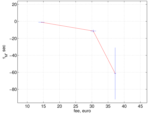
Figure 18: Averaged fee (X-axis) and $\tau_{M}$ (Y-axis). Three points with error bars are for (by increased $fee$ value) fast, medium and slow types of Investors. Averaging is done over all stocks.

We realize that the division into groups of Investors is voluntary and is not covered by the model described in (7). This effect should be accounted in future developments.

Concluding the test of inequality (9) we see that in average market preserves the trend arbitrage requirements. In particular situations, however, given on page 2, an arbitrage is still possible.

4.2 Tick size and Specialists activity

4.2.1 Formula

Tick size, $dp$, is another important ingredient of the trend arbitrage equation. Let us use similar arguments about trend arbitrage (like used in section 2, ”Trend arbitrage”). Consider the same situation when ask prices move with up-trend (see Figure 2). If to assume that the price is updated every time when the expected price becomes larger than the current one by tick-size, the number of price updates should be:

$$N_{u}\sim\frac{\Delta p}{dp}=\frac{|\mu|\Delta T}{dp}\textrm{ and therefore }$$

$$dp\sim|\mu|\frac{\Delta T}{N_{u}}=|\mu|\tau_{u}$$ (8)

where, $\Delta T$ is duration of the trend, $\Delta p$ is price change and $N_{u}$ is number of ask updates during same period and $\tau_{u}$ is average update time alongside the trend. Which sign must be used in the relationship, ($=$) or strict inequality, is difficult to say because the spread compensates for low update frequency. Therefore we leave ($\sim$)-sign.

4.2.2 Analysis

Data demonstrate, that distribution of $\mu\cdot\tau_{u}$ follows normal distribution with some tails, which can be attributed to some inefficiency in the process, see Figure 20. Tick size is covered within $3\sigma$ of the distribution. It means that price update happens more often than necessary giving almost no chance for trend arbitrage.

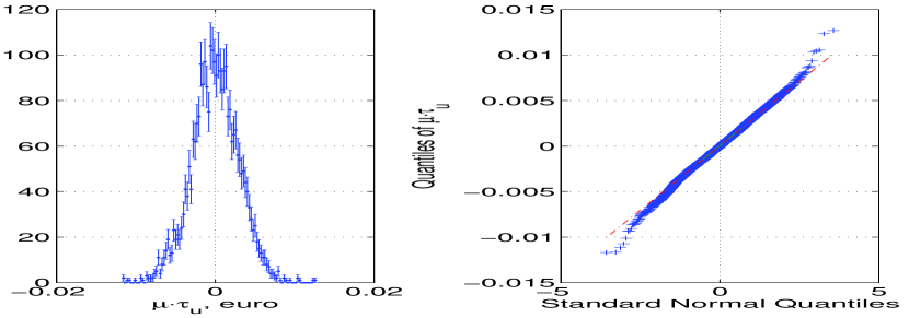
Figure 20: Distribution of $\mu\cdot\tau_{u}$ for ABN-AMRO (left) with fitted Normal p.d.f.. Right plot is quantile plot of the same value versus normal quantile.

Figure 22 plots the $3\sigma(\mu\tau)/dp$ of $\mu\tau$ distributions for all stocks under consideration. We see that with few exceptions update frequency is such that $3\sigma$ of $\mu\tau$ is within tick size which confirms our proposition.

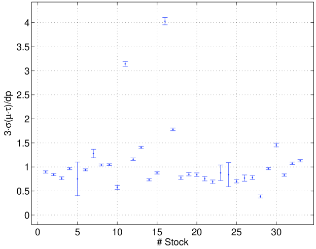
Figure 22: $\frac{3\sigma(\mu\tau)}{dp}$ of $\mu\tau$ distributions. Some anomalies of unknown origin show-up for two German stocks # 11 and 16 (Allianz and SAP, respectively).

The general conclusion is that the tick size closely influences trading activity by pushing Specialists to update their future price view. The larger tick size, the less Specialist is motivated to do so. We see such pattern for some stocks of Euronext. When their price crosses 50 $euros$ boundary  the price update frequency drops accordingly.

Following trend arbitrage logic, if the tick size is small but exchange or trading systems are slow (e.g. Specialists trading on floor), then the $\frac{3\sigma(\mu\tau)}{dp}$ must be larger than 1. If this is not compensated with larger spread the arbitrage exists.

By substituting (8) into (7) we obtain the following:

$$\frac{Spr-dp}{|\mu|}\geq\tau_{M}+\frac{fee}{|\mu|}$$ (9)

Performing the same measurement of $\tau_{M}$ as in section 4.1.1 we find that the distinction between exchanges is almost removed and is now ranges between 0.6 and 1.2 second (see Figure 24 and Table 6. Taking $dp=0.01$ $eur$ (and $0.05$ $eur$ for some stocks of Euronext) and fitting edge of ($\frac{Spr-dp}{|\mu|}$,$\frac{1}{|\mu|})$-distribution as it was done before in section 4.1.2 reveals (see Figure 26) that tick size, $dp$, absorbs both $\tau_{S}$ and (probably) $\tau_{M}$, therefore, reducing (9) to the following:

$$Spr-dp\geq\tau_{M}\cdot\mu+fee$$ (10)

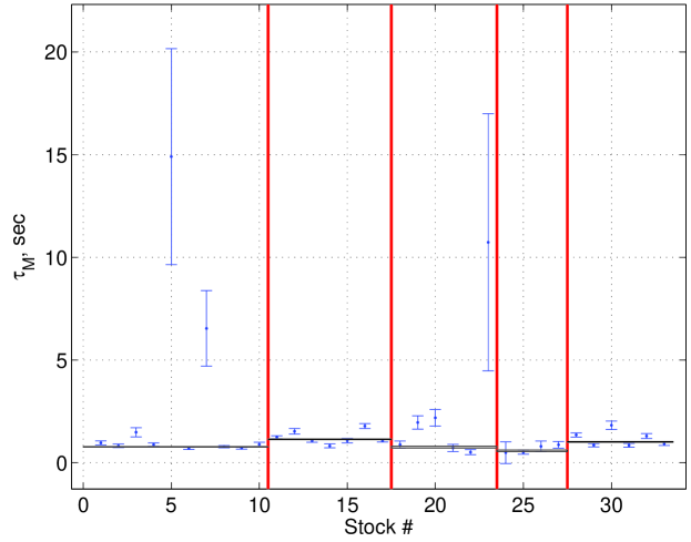
Figure 24: $\tau_{M}$ values measured per stock (numbered from 1 to 33) using (9). Results are sorted by exchanges where stocks are traded in bands separated by vertical lines. Exchanges (left to right) are Amsterdam (NLD), Frankfurt (GER), Madrid (SPA), Milano (ITL) and Paris (FRA). Horizontal lines indicate range of $\tau_{M}$ for each exchange.

Table 6: Exchange averages of measured $\tau_{M}$. Eq (9) is used.

Exchange	$\tilde{\tau_{M}}$
Amsterdam (NLD)	0.79 $\pm$ 0.03
Frankfurt (GER)	1.15 $\pm$ 0.03
Madrid (SPA)	0.8 $\pm$ 0.1
Milano (ITA)	0.6 $\pm$ 0.1
Paris (FRA)	1.04 $\pm$ 0.04

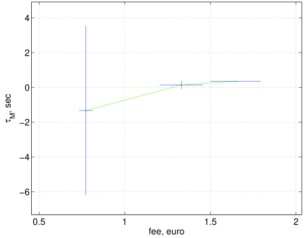
Figure 26: Averaged fee (X-axis) and $\tau_{M}$ (Y-axis). Three points with error bars are for (by increased $fee$ value) slow, medium and fast types of Investors. Averaging is done over all stocks.

We may conclude from this result, that (8) absorbs all stock specific and (probably) exchange-wide latencies information. In fact, all results described in this article should be confirmed from actual hardware response, i.e. direct measurement of all latencies within exchange and traders computers/software.

4.2.3 Simulation: Trends in Random walk model and return-trend duality

A simplified model of price evolution has been implemented to understand empirical results. The price increment of this model follows $dS=\sigma dW$. Trend search algorithm (given in section 3.2) is imposed to generated price time series. Trends found with that procedure are stored in the same fashion as we did for real data.

Two important points have to be mentioned:

• The model assumes generation of prices at equal time intervals, i.e. trading activity is not simulated and

• Spread is assumed to be constant and is not dependent on the trend;

In particular, the model reproduces Normal distribution of $|\mu|\tau_{u}$ for all tracks. This leads to an idea that the description of price evolution with some random walk model is equivalent to description of price via trends, which also can be stochastic .

To be more specific let us consider some stochastic model describing price dynamics, like Black-Scholes model, $BS(\mu,\sigma;\epsilon)$ with growth rate, $\mu$, volatility, $\sigma$, and $\epsilon$, some value to cut the trend, like $n$ in (6), as parameters. Then, there is a homeomorphic transformation in parametric space into another model describing same price dynamics in terms of trends, $T(\mu,\Delta T;q)$, with trend slope, $\mu$, trend duration, $\Delta T$, and quality, $q$, as parameters. Quality, $q$, characterizes amount of fluctuations around trend (spread dynamics).

4.2.4 Beta

Looking closer to relationship between $\frac{\tilde{Spr}}{\mu}$ and $\tau_{u}=\frac{\Delta T}{N_{u}}$, Figure 28,

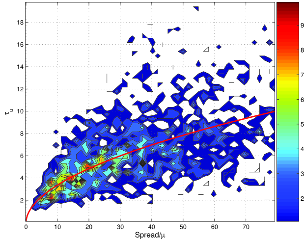
Figure 28: Dependence of $\tau_{u}$ on $\frac{\tilde{Spr}}{\mu}$ for ABN-AMRO. Solid line indicates $x^{0.625}$ function.

we can find strong relationship:

$$\frac{\tilde{Spr}}{\mu}=\tau_{u}^{1+\beta}+\eta,$$ (11)

where $\beta$ is stock dependent and ranges between 0.3 and 1.1, see Figure 30, and $\eta$ is random Wiener process scaled roughly as $\tau$.

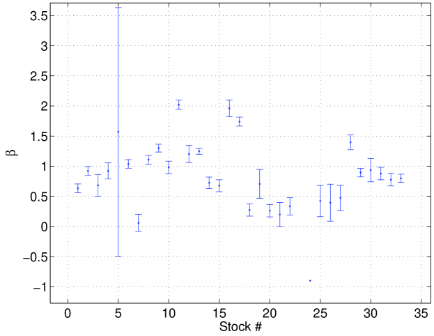
Figure 30: $\beta$ for all stocks.

Indeed, the distribution of difference $\frac{\tilde{Spr}}{\mu}-\tau_{u}^{1+\beta}$ has a peak around zero and fits to Normal p.d.f. where part of distribution is cut due to trend arbitrage, which plays role of natural constrain for price generaion process (11). $\beta$ is found through two-step procedure:

• slices in $\frac{Spr}{|\mu|}$ are fit to Normal p.d.f., $N(m_{\tau},s)$;

• $m$ are fit to $\frac{Spr}{|\mu|}=m_{\tau}^{1+\beta}$

It is difficult to interpret meaning of this relationship, because dimensionalities of l.h.s and r.h.s. of equation (11), [$sec$] and [$sec^{\beta}$], are different. There is some reference model though [SABR], which suggests fractionality of return process:

$$dF=aF^{\beta}dW_{1};\textrm{ }da=\nu adW_{2};\textrm{ }dW_{1}dW_{2}=\rho dt$$ (12)

The main difference, however, with the mentioned result is that SABR-model describes process of last prices, while equation (11) describes bid-ask update. The relationship between bid-ask update process and trade process is subject of the next article.

5 Conclusions and prospects

The presented analysis has demonstrated importance of analysis of short-term trends as it gives better insight into micro-dynamics of the market.

Using simple mechanistic arguments the trend arbitrage inequality is developed. Empirical tests prove the inequality to hold. The inequality sets limit on bid-ask spread which is determined by the latencies of exchange and trading systems and by some costs. These latencies can also be identified directly by measuring delay between sending time of the order from traders computer and appearance of this order in the exchange book.

Using same arguments, the tick size is related to frequency of price update by Specialist. Analysis of trend inequality with data allowed us to measure latencies of exchange

Flat distribution of probability of $\chi^{2}_{t}$ of trend fit demonstrates that the spread bears instant information about price uncertainty in the process of price measurement. Indeed, from the point of view of Investor the next last price will be within the current bid-ask spread.

Structure of trend arbitrage is in general captured correctly. In particular, it allows to see division of market participants by their speed.

Further analysis suggests some strong relationship between spread, trend and time of trades update. Although dimensionality problem of the equation remains, the theoretical explanation of this phenomenon is still waiting to appear.

The final conclusion is that the price evolution can be equally described through random walk or trends. However, market participants induce such spread dynamics as the trend exists and they limit their actions to conform trend arbitrage requirement.

In the future research, we plan to investigate relationship between price update and $trading$ processes using the same type of analysis of trend associated information. Some model development will take place as well.

References

- [Bondarenko] O.Bondarenko, ”Competing market makers, liquidity provision, and bid-ask spreads”. Journal of Financial Markets, 4(2001) 269-308.
- [Derman] E.Derman, ”The perception of time, risk and return during periods of speculation”, Quantitative Finance, V.2 2002) 282-296.
- [Durlauf] S.Durlauf and P.Phillips (1988), ”Trends versus Random Walks in Time Series Analysis”, Econometrica, Volume 56, Issue 6 (Nov. 1988), 1333-1354.
- [SABR] P.S.Hagan, D.Kumar, A.S.Lesniewski and D.E.Woodward, ”Managing smile risk”, Wilmott Magazine, Oct 2002.
- [Roll] R.Roll, ”A simple implicit measure of the effective bid-ask spread in an efficient market”, Journal of Finance, Vol. 39, No. 4 (Sep., 1984) , pp. 1127-1139.
- [Schleifer] Andrei Shleifer, ”Inefficient Markets”. Clarendon Lectures. Oxford University Press.
- [Smith et.al.] E.Smith, J.D.Farmer, L.Gillemot and S.Krishnamurthy, ”Statistical theory of the continuous double auction”. arXiv:con-mat/0210475, 22 Oct 2002.
- [Wiki] see for example http://en.wikipedia.org/wiki/Linear_regression