Shape changes and motion of a vesicle in a fluid using a lattice Boltzmann model

Abstract

We study the deformation and motion of an erythrocyte in fluid flows via a lattice Boltzmann method. To this purpose, the bending rigidity and the elastic modulus of isotropic dilation are introduced and incorporated with the lattice Boltzmann simulation, and the membrane-flow interactions on both sides of the membrane are carefully examined. We find that the static biconcave shape of an erythrocyte is quite stable and can effectively resist the pathological changes on their membrane. Further, our simulation results show that in shear flow, the erythrocyte will be highly flattened and undergo tank tread-like motion. This phenomenon has been observed by experiment very long time ago, but it has feazed the boundary integral and singularity methods up to the present. Because of its intrinsically parallel dynamics, this lattice Boltzmann method is expected to find wide applications for both single and multi-vesicles suspension as well as complex open membranes in various fluid flows for a wide range of Reynolds numbers.

Vesicle whose membrane consists of lipid bilayer is essential to the function of biological systems Fung97 . Erythrocyte is the most important kind of vesicles. In the past 30 years, the dynamics of vesicle has received particular attention Ou-Yang87 ; Lipowsky96 ; PozrikidisBook92 ; Secomb01 . It has been recognized that the equilibrium shape can be obtained by minimizing the bending energy of the membrane Ou-Yang87 . However, the studies on the unsteady states lag behind, mainly because of the numerical difficulty on capturing the coupling between the membrane and ambient fluids while the vesicle is deforming and moving under the hydrodynamic forces exerted on both sides of its elastic membrane Lipowsky96 . When the vesicle is very close to a solid static boundary and the Reynolds number is very small, lubrication theory has been extended to the study Secomb01 . Recently, the deformations of vesicles in the approximation of Stokes flow has been extensively studied by the boundary integral and singularity methods PozrikidisBook92 ; Lipowsky96 , which has a limitation imputed to the absence of numerical smoothing and accuracy of regridding Pozrikidis03 so that it can not describe the highly flattened tank-treading shapes.

Erythrocytes in large blood vessels, which have larger Reynolds numbers, not only affect the viscosity of the fluid Stoltz99 , but also often subject to pathological changes of their membranes due to the large shear stress Gallucci99 . This calls for computing models for deformations of vesicles, particularly with inhomogeneous membrane, in fluid flow with a wide range of Reynolds numbers. Moreover, considering the numerical complexity of the vesicle deformations and multi-vesicle suspensions, and the recent development of computational technique, especially on the PC clusters and internet grid computing, it is most desirable that the numerical models are intrinsically parallel. The lattice Boltzmann method (LBM) McNamara88 ; Qian92 has localized kinetic nature which is not only intrinsically parallel but also easy to capture the interaction between a fluid and a small segment of a deformable boundary. In the past fifteen years, the LBM has been recognized as an alternate method for computational fluid dynamics, especially in the areas of complex fluids such as particle suspension flow Ladd01 , binary mixture Gunst91 and blood flow Buick02 . However, applicability of LBM on the vesicle deforming and moving remains an open problem. A crucial difficulty is the physics that the membrane is viscoelstic and area-unchangeable while the total volume of the vesicle keeps a constant. Numerically, the viscoelstic property demands that the boundary condition and the hydrodynamic force should be accurately treated even in a very small segment. In two-dimensional problems, area- and volume- unchangeability are reduced to inextensibility of the one-dimensional membrane and area-unchangablility of the area surrounded by the one-dimensional membrane. In this Letter we develop a lattice Boltzmann model in which the elastic properties, length constrain of the membrane and volume constrain on area of vesicle incorporated in a discrete way with a boundary treatment for moving boundaries.

We choose to work with the D2Q9 model on a two-dimensional square lattice with nine velocities Qian92 . Let $f_{\alpha}({\bf x},t)$ be the non-negative distribution function which can be thought as the number of fluid particles at site ${\bf x}$, time $t$, and possessing one of the nine velocities ${\bf e}_{\alpha}$. The distribution function evolves according to a Boltzmann equation that is discrete in both space and time,

$$f_{\alpha}({\bf x}+{\bf e}_{\alpha},t+1)-f_{\alpha}({\bf x},t)=-\frac{1}{\tau}(f_{\alpha}-f_{\alpha}^{eq}).$$ (1)

The density $\rho$ and macroscopic velocity ${\bf u}$ are defined by

$$\rho=\sum_{\alpha}f_{\alpha},\ \ \ \rho{\bf u}=\sum_{\alpha}f_{\alpha}{\bf e}_{\alpha}.$$ (2)

Here, the equilibrium distribution function $f_{\alpha}^{eq}$ depends only on the local density $\rho$ and flow velocity ${\bf u}$. The pressure and the viscosity are defined by the equations $p=c_{s}^{2}\rho$ with $c_{s}^{2}=1/3$ and $\nu={(2\tau-1)/6}$, respectively Qian92 .

The membrane of the erythrocytes has bending rigidity potential, which can be written as Ou-Yang87 ; PozrikidisBook92

$$\phi_{B}=\frac{1}{2}k_{B}\int{k^{2}\mathrm{d}l},$$ (3)

where $k_{B}$ is the bending modulus, $k$ and $l$ are the curvature and the arc length of the membrane, separately. Biomembranes are formed by a lipid bilayer, which is viscoelastic. The erythrocyte viscoelasticity is usually assumed to be Kelvin-Voigt Evans76 and described by

$$T_{mn}=2\eta\dot{\varepsilon}_{mn},$$ (4)

where $T_{mn}$ is the viscous stress, $\dot{\varepsilon}_{mn}$ and $\eta$ are the strain rate and the viscous coefficient of the membrane. The viscoelasticity of the membrane does not change the static shapes of erythrocytes.

Numerically, the membrane of a two-dimensional erythrocyte is discretized into equilength segments. We implement a no-slip boundary condition and compute the hydrodynamic forces on both sides of each segment according to the scheme proposed recently Li2004b . The isotropic dilation can be described by adopting an in-plane potential $\phi_{k}$ between neighboring segments as

$$\phi_{k}=\frac{1}{2}{k_{k}\sum_{i=1}^{N}(l_{i}-l_{0})^{2}},$$ (5)

where $k_{k}$ is the elastic coefficient of the membrane, $l_{0}$ and $l_{i}$ are the original and simulated length of segment $i$ respectively. Pozrikidis has already shown that the transverse shear tension due to the bending energy can be computed as PozrikidisBook92

$$F^{B}=k_{B}\frac{\partial k}{\partial l}.$$ (6)

The force exerted on segment $i$ on the normal direction due to the bending energy is

$$F_{i}^{B}=k_{B}\frac{k_{i+1}-k_{i}}{l_{i}},$$ (7)

where $k_{i+1}$ and $k_{i}$ are the curvatures of the membrane at segments $i+1$ and $i$, respectively. The membrane viscous resistance on the normal direction on segment $i$ is

$$F^{r}_{i}=-\eta(v_{i+1,n}-v_{i,n}),$$ (8)

where $v_{i+1,n}$ and $v_{i,n}$ is the velocity of segments $i+1$ and $i$ along the normal direction of segment $i$, separately.

The translation of each segment is updated at each Newtonian dynamics time step according to the sum of all the forces on the segment by using a so-called half-step ‘leap-frog’ scheme Allen1987 .

The membrane parameters are set to be $k_{B}=1.8\times 10^{-12}$ $\mathrm{dyn\cdot cm}$ PozrikidisBook92 and $\eta=1.0\times 10^{-5}$ $\mathrm{dyn\cdot s/cm}$ Evans76 . The blood serum is usually assumed to be Newtonian and has a viscosity $\nu=0.01$ $\mathrm{cm^{2}/s}$ and density $\rho=1.00$ $\mathrm{g/cm^{3}}$ PozrikidisBook92 . The fluid inside the erythrocytes is also assumed to be serum too. The thickness and the density of the membrane are set to be 0.02 $\mathrm{\mu m}$ and 1.00 $\mathrm{g/cm^{3}}$, respectively Oka88 . The cross-membrane pressure drop of an erythrocyte can be expressed by the chemical potential drop Walter95

$$\Delta\mu=RT\ln(\frac{p_{\mathrm{out}}}{p_{\mathrm{in}}}),$$ (9)

where $p_{\mathrm{out}}$ and $p_{\mathrm{in}}$ are the pressure outside and inside the erythrocyte, separately. The temperature is set to the human body temperature $37^{o}$ C. The longer axis of an erythrocyte is set to 3.9 $\mu$m and the according shorter axis is 0.4 $\mu$ m Oka88 . The elastic modulus of isotropic dilation is $k_{k}=500$ $\mathrm{dyn/cm}$ PozrikidisBook92 .

Figure 1: The static profiles of an erythrocyte for $\Delta\mu$ = 2.71 ($\square$), 2.97 ($\bigcirc$), 3.39 (${\color[rgb]{0,1,0}\star}$), and 3.82 (${\color[rgb]{0,0,1}\triangle}$) $\times 10^{-5}$J/mol calculated from lattice Boltzmann simulations (symbols) together with those from a shooting method Pozrikidis02 (lines). $x$ and $y$ are normalized by the total length of the membrane.

The simulation domain consists of $200\times 80$ lattice units. We have tested that when the width is greater than 200 lattice units, increase of width dose not affect the simulation results if the boundary conditions of both left and right sides are periodic. Initially, the fluid was homogeneous and steady. A circular membrane placed at the center of the square without stretching was discretized into $N=100$ segments. The radius of the initial circular membrane was 20 lattice units. The length in each lattice unit corresponded to 0.14 $\mathrm{\mu m}$. The relaxation time $\tau$ was fixed to be 0.75, resulting in $1.69\times 10^{-9}$ s for each time step. The initial density of the fluid inside and outside the close membrane was set to be one lattice Boltzmann unit. The other non-dimensional quantities relevant to lattice Boltzmann simulations could be computed correspondingly. In the simulation, the fluid in the square of $6\times 6$ lattice units at the center of the system was pumped out with a speed of $1.69\times 10^{-9}$ $\mathrm{g/s}$, i.e., $1/1000$ per time-step, until the predetermined chemical potential drop was reached, the mass inside the erythrocyte is then remained constant for the remainder of the simulation.

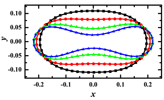
Fig. 1 shows the profiles of an erythrocyte with different chemical potential drops $\Delta\mu$ together with that of a shooting method Pozrikidis02 . As $\Delta\mu$ increases, the erythrocyte deforms from a circle to an ellipse, and into an biconcave shape. Excellent agreement can be found between the two methods. In order to further characterize the agreement, we have also computed the relative global error $\sigma$ of the curvature of the membrane between the two methods, defined by

$$\sigma={\sum\limits_{i=1}^{N}(k_{i}-k^{\prime}_{i})^{2}}/{\sum\limits_{i=1}^{N}k_{i}^{{}^{\prime}2}},$$ (10)

where $k_{i}$ and $k^{\prime}_{i}$ are the curvatures at segment $i$, calculated from lattice Boltzmann simulations and the shooting method Pozrikidis02 , respectively. We found that the relative global error was less than $10^{-5}$.

Figure 2: Static profiles of erythrocytes for bending modulus varying according to Eq. (11). (a) For small chemical potential drop $\Delta\mu$ = $4.24\times 10^{-6}$ J/mol, lines with $\square,{\color[rgb]{1,0,0}\bigcirc},{\color[rgb]{0,0,1}\triangle},{\color[rgb]{0,1,0}\diamondsuit}$ correspond to $n=2,3,4,5$, respectively. (b) and (c) Erythrocyte profiles for larger chemical potential drops. $\Delta\mu$ = 0.68, 0.68, 1.87, 1.10, 1.18 and 1.10 ($\times 10^{-5}$J/mol) for $n=2,4,3,5,19,20$.

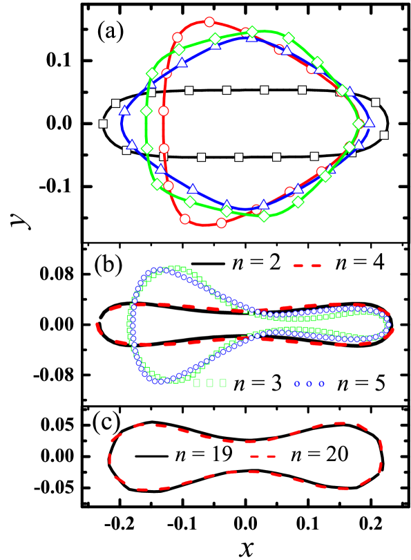
Due to high values of shear stress in the large arteries or in cases of oxidant injury Gallucci99 , erythrocyte membranes can be pathologically damaged so that the bending rigidity modulus becomes non-uniform. To study the effect on the shapes of the erythrocytes, we performed numerical simulations with bending modulus changing periodically along the membrane

$$K_{B}=K_{0}\left[\delta+(1-\delta)\cos^{2}(n\pi l^{\prime})\right],0\leq l^{\prime}<1,$$ (11)

where $\delta$ is a constant, $l^{\prime}$ is the normalized arc length of the membrane, and $n$ is an integer. The simulation results for $\delta=0.1$ are shown in Fig. 2. For small chemical potential drop, say $\Delta\mu\leq 4.24\times 10^{-6}$ J/mol, the shape of the erythrocyte exhibits the same symmetry of $K_{B}$. Remarkably, when $\Delta\mu$ is large enough, all erythrocytes, with different bending modulus, become biconcave shapes, i.e., the biconcave shapes can effectively resist the perturbations. We note that the perturbations are quite large as the minimum of $K_{B}$ is only $10\%$ of its original value. Further, erythrocyte profiles for perturbation wave numbers of the same parity are very similar to each other. As shown in Fig. 2 (b), the difference between the profiles for $n=3$ and $n=5$, or that between $n=2$ and $n=4$ is almost indistinguishable whereas the discrepancy between the cases of $n=2$ and $n=3$ is clear. When the wave number $n$ is large enough, the difference for odd and even $n$ becomes very small as shown in Fig. 2 (c). The chemical potential drop needed to collapse an erythrocyte is smaller for an even $n$ than that for an odd $n$, this difference becomes vanishingly small as $n$ increases.

Figure 3: Erythrocyte deforming and moving in shear flow. (a) Orientation angle as a function of the swelling ratio $\Gamma$ with the shear rate $\gamma=7481\mathrm{s}^{-1}$,together with the results of Green function and KS theory Beaucourt04 . (b) Tank tread frequency $f$ plotted against the shear rate $\gamma$. $\square$ and $\bigcirc$ correspond to lattice Boltzmann simulation and experimental results Fischer78 , respectively. The frequency of lattice Boltzmann simulation is multiplied by $2\pi$. Inset: a terminal snapshot of an erythrocyte in a shear flow for $\gamma=598$ and 449 $\mathrm{s^{-1}}$.

Now, we performed simulations of an erythrocyte deforming and moving in a shear flow. According to the KS theory Beaucourt04 , two parameters relevant to the tank tread-like motion of an erythrocyte are the swelling ratio

$$\Gamma=4\pi S/P^{2},$$ (12)

and the viscosity ratio

$$r=\rho_{in}\nu_{in}/\rho_{out}\nu_{out},$$ (13)

where $S$ and $P$ are the area and the girth of a two-dimensional erythrocyte, $\rho$ and $\nu$ are the density and kinematic viscosity of the fluid inside or outside the erythrocyte, marked by subscripts $in$ and $out$, respectively. In our simulations $r\approx 1.0$ PozrikidisBook92 . At first, we pumped out some fluid inside the erythrocyte until the chemical potential reached a certain value. Consequently, the upmost and lowest layer in the simulation domain has a rightward and leftward velocity, respectively, with a same magnitude to produce a simple shear flow. Meanwhile, the area of the erythrocyte was kept nearly invariable by minus increased mass

$$\Delta d=\frac{S\bar{\rho}-S_{0}\bar{\rho}_{0}}{M}$$ (14)

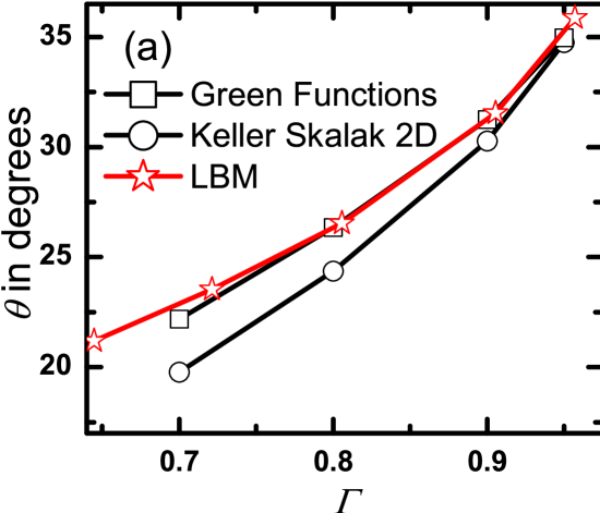
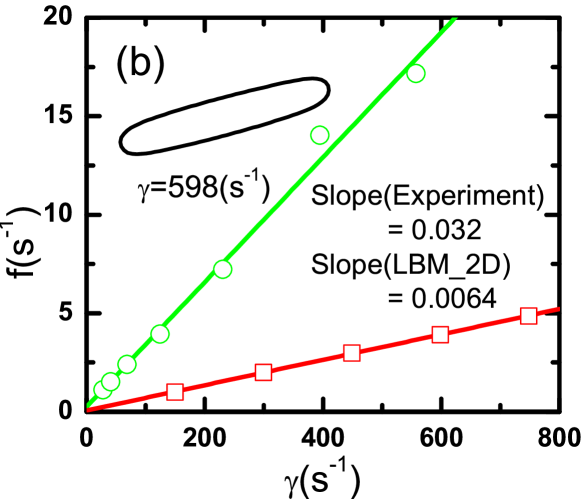
from every fluid node inside the erythrocyte, where $S_{0}$ and $S$ are the areas of the erythrocyte before and after adding a shear flow, $\bar{\rho}_{0}$ and $\bar{\rho}$ are the average densities inside the erythrocyte before and after adding a shear flow, $M$ is the number of fluid nodes inside the erythrocyte. According to the KS theory, the orientation angle of an erythrocyte moving in a shear flow will vary with $\Gamma$. From Fig. 3 (a), we can see that our simulation results agree with the results calculated by Green functions Beaucourt04 very well when the swelling ratio $\Gamma>0.8$. In fact, when $\Gamma<0.8$, the shape of the erythrocyte without any shear flow will be concave and its terminal shape with a shear flow will be protuberant, but different from ellipsoid. In Fig. 3 (b), the swelling ratio $\Gamma=0.418$, the erythrocytes undergo tank tread-like motion, consistent with the famous experimental observation by Fischer and Schmidt-Schönbein Fischer78 . The final shape of the erythrocyte for $\gamma=598$ $\mathrm{s^{-1}}$ are shown in the inset of Fig. 3 (b). Numerically we find that the erythrocyte deformed from original biconcave shape into a highly flattened shape, which the the boundary integral and singularity methods can not get despite two-dimensional or three-dimensional calculation Pozrikidis03 . We have computed the tank tread frequency with respect to the shear rate for $\Gamma=0.418$. The result is displayed in Fig. 3 (b) together with the experimental one Oka88 . It is clear that our two-dimensional simulation result has the same linear behavior as the frequency of experiment. Because the swelling ratio of a cross section of three dimensional biconcave erythrocytes may continuously increases to one, our two-dimensional simulation is only for one certain cross section of three-dimensional, for example the center cross section.

To summaries, we have developed a lattice Boatsman model to simulate vesicle deforming and moving in various fluid flows for a wide range of Reynolds numbers. The results show that the static biconcave shape is rather steady that it can effectively resist pathological changes on the membranes. In a shear flow, an erythrocyte will deform from biconcave shape into a highly flattened one. Considering the intrinsic parallelity of the lattice boltzmann method, this scheme may have good prospects for the simulations of various vesicles deforming and moving in the vessel or capillary.

This work was partially supported by the National Natural Science Foundation of China through projects No. 10447001 and 10474109, Foundation of Ministry of Personnel of China and Shanghai Supercomputer Center of China.

References

- (1) Y.C. Fung, Biomechanics Circulation (Springer-Verlag, Berlin, 1997).
- (2) Z.C. Ou-Yang and W. Helfrich, Phys. Rev. Lett. 59, 2486 (1987); Q. Du, C. Liu, R. Ryham, and X. Wang, J. Comput. Phys. 198, 450 (2004); M. Iwamoto and Z.C. Ou-Yang, Phys. Rev. E 93, 206101 (2004); R. Lipowsky and E. Sackmann, Structure and Dynamic of Membranes (Elsevier, Amsterdam, 1995).
- (3) M. Kraus, W. Wintz, U. Seifert, and R. Lipowsky, Phys. Rev. Lett. 77, 3685 (1996).
- (4) T.W. Secomb, R. Hsu, and A.R. Pries, Am. J. Physiol. Heart Circ. Physiol. 281, 629 (2001).
- (5) C. Pozrikidis, Modeling and Simulation of Capsules and Biological Cells (Boca Raton: Chapman & Hall/CRC, 2003).
- (6) C. Pozrikidis, J. Fluid Mech. 440, 269 (2001); C. Pozrikidis, Ann. Biomed. Eng. 31, 1 (2003); C.D. Eggleton and A.S. Popel, Phys. Fluids 10, 1834 (1998).
- (7) J.F. Stoltz et al., Clin. Hemorheol. Micro. 21, 201 (1999).
- (8) M.T. Gallucci, et al., Clin. Nephrology 52, 239 (1999).
- (9) G.R. McNamara and G. Zanetti, Phys. Rev. Lett. 61, 2332 (1988); S.Y. Chen, H.D. Chen, D.O. Martinez, and W.H. Matthaeus, Phys. Rev. Lett. 67, 3776 (1991); S. Succi, The Lattice Boltzmann Equation for Fluid Dynamics and Beyond (Oxford: Clarendon Press, 2001).
- (10) Y.H. Qian, D. d’Humiéres, and P. Lallemand, Europhys. Lett. 17, 479 (1992).
- (11) A.J.C. Ladd and R. Verberg, J. Stat. Phys. 104, 1191 (2001); C.k. Aidun, Y. Lu, and E. Ding, J. Fluid Mech. 373, 287 (1998); D.R. Noble and J.R. Torczynski, Int. J. Mod. Phys. C 9, 1189 (1998); O. Filippova and D. Hanel, Comput. Fluids. 26, 697 (1997); H.B. Li, H.P. Fang, Z.F. Lin, S.X. Xu, and S.Y. Chen, Phys. Rev. E 69, 031919 (2004).
- (12) A.K. Gunstensen, D.H. Rothman, S Zaleski, and G. Zanetti, Phys. Rev. A 43, 4320 (1991); X.W. Shan and H.D. Chen, Phys. Rev. E 47, 1815 (1993); M.R. Swift, S.E. Orlandini, W.R. Osborn W R, and J.M. Yeomans, Phys. Rev. Lett. 75, 830 (1995); A.G. Xu, G. Gonnella, and A. Lamura, Physica A 331, 10 (2004).
- (13) J.M. Buick, et al., Biomed. Pharmacother 56, 345 (2002); M. Krafczyk, M. Cerrolaza, M. Schulz, and E. Rank, J. Biomech. 31, 453 (1998); H.P. Fang, Z.W. Wang, Z.F. Lin, and M.R. Liu, Phys. Rev. E 65, 051925 (2002); A.G. Hoekstra, J. van‘t Hoff, A.M.M. Artoli, and P.M.A. Sloot, Lect. Notes Comput. Sci. 2657, 997 (2003); M. Hirabayashi, M. Ohta, D.A. Rüfenacht, and B. Chopard, Phys. Rev. E 68, 021918 (2003); C. Migliorini, et al., Biophys. J. 83, 1834 (2002); M.M. Dupin and I. Halliday, J. of Phys. A 36, 8517 (2003).
- (14) E.A. Evans and R.M. Hochmuth, Biophys. J. 16, 1 (1976).
- (15) H.B. Li, X.Y. Lu, H.P. Fang, and Y.H. Qian, Phys. Rev. E 70, 026701 (2004).
- (16) M.P. Allen and D.J. Tildesley, Computer Simulation of Liquid (Clarendonn, 1987).
- (17) Syoten Oka, Biorheology (Science Press, Peking, in Chinese, translated by Y.P Wu, Z.C. Tao, et al., 1988).
- (18) G. Walter, N. Ludwig, and S. Horst, Thermodynamics and Statistical Mechanics (Springer, 1995).
- (19) C. Pozrikidis, J. Eng. Math. 42, 157 (2002).
- (20) J. Beaucourt, F. Rioual, T. Séon, T. Biben, and C. Misbah, Phys. Rev. E 69, 011906 (2004).
- (21) T.M. Fischer and H. Schmid-Schnbein, Red Cell Rheology (Springer-Verlag, Berlin, 1978).