Inverse cubic law of index fluctuation distribution in Indian markets

Abstract

One of the principal statistical features characterizing the activity in financial markets is the distribution of fluctuations in market indicators such as the index. While the developed stock markets, e.g., the New York Stock Exchange (NYSE) have been found to show heavy-tailed return distribution with a characteristic power-law exponent, the universality of such behavior has been debated, particularly in regard to emerging markets. Here we investigate the distribution of several indices from the Indian financial market, one of the largest emerging markets in the world. We have used tick-by-tick data from the National Stock Exchange (NSE), as well as, daily closing data from both NSE and Bombay Stock Exchange (BSE). We find that the cumulative distributions of index returns have long tails consistent with a power-law having exponent $\alpha\approx 3$, at time-scales of both 1 min and 1 day. This “inverse cubic law” is quantitatively similar to what has been observed in developed markets, thereby providing strong evidence of universality in the behavior of market fluctuations.

I Introduction

Financial markets can be viewed as complex systems with a large number of interacting components that are subject to external influences or information flow. Physicists are being attracted in increasing numbers to the study of financial markets by the prospect of discovering universalities in their statistical properties Mantegna and Stanley (1999); Bouchaud and Potters (2003); Chatterjee and Chakrabarti (2006). This has partly been driven by the availability of large amounts of electronically recorded data with very high temporal resolution, making it possible to study various indicators of market activity. Among the various candidates for market-invariant features, the most widely studied are the distributions of fluctuations in overall market indicators such as market indices.

To study these fluctuations such that the result is independent of the scale of measurement, we define the logarithmic return for a time scale $\Delta t$ as,

$$R(t,\Delta t)\equiv\ln{I(t+\Delta t)}-\ln{I(t)},$$ (1)

where $I(t)$ is the market index at time $t$ and $\Delta t$ is the time-scale over which the fluctuation is observed. Market indices, rather than individual stock prices, have been the focus of most previous studies as the former is more easily available, and also gives overall information about the market. By contrast, individual stocks are susceptible to sector-specific, as well as, stock-specific influences, and may not be representative of the entire market. These two quantities, in fact, characterize the market from different perspectives, the microscopic description being based on individual stock price movements, while the macroscopic point of view focusses on the the collective market behavior as measured by the market index.

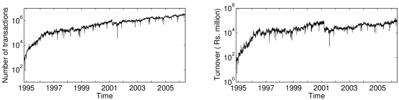
Figure 1: Time evolution of the National Stock Exchange of India from $1994-2006$ in terms of (left) the total number of trades and (right) the total turnover (i.e., traded value).

The importance of interactions among stocks, relative to external information, in governing market behavior has emerged only in recent times. The earliest theories of market activity, e.g., Bachelier’s random walk model, assumed that price changes are the result of several independent external shocks, and therefore, predicted the resulting distribution to be Gaussian Bachelier (1900). As an additive random walk may lead to negative stock prices, a better model would be a multiplicative random walk, where the price changes are measured by logarithmic returns Osborne (1964). While the return distribution calculated from empirical data is indeed seen to be Gaussian at long time scales, at shorter times the data show much larger fluctuations than would be expected from this distribution Fama (1965). Such deviations were also observed in commodity price returns, e.g., in Mandelbrot’s analysis of cotton price, which was found to follow a Levy-stable distribution Mandelbrot (1963). However, it contradicted the observation that the distribution converged to a Gaussian at longer time scales. Later, it was discovered that while the bulk of the return distribution for the S&P 500 index appears to be fit well by a Levy distribution, the asymptotic behavior shows a much faster decay than expected. Hence, a truncated Levy distribution, which has exponentially decaying tails, was proposed as a model for the distribution of returns Mantegna and Stanley (1995). Subsequently, it was shown that the tails of the cumulative return distribution for this index actually follow a power-law,

$$P_{c}(r>x)\sim x^{-\alpha},$$ (2)

with the exponent $\alpha\approx 3$ (the “inverse cubic law”) Gopikrishnan et al. (1998), well outside the stable Levy regime $0<\alpha<2$. This is consistent with the fact that at longer time scales the distribution converges to a Gaussian. Similar behavior has been reported for the DAX, Nikkei and Hang-Seng indices Lux (1996); Gopikrishnan et al. (1999). These observations are somewhat surprising, although not at odds with the “efficient market hypothesis” in economics, which assumes that the movements of financial prices are an immediate and unbiased reflection of incoming news and future earning prospects. To explain these observations various multi-agent models of financial markets have been proposed, where the scaling laws seen in empirical data arise from interactions between agents Lux and Marchesi (1999). Other microscopic models, where the agents (i.e., the traders comprising the market) are represented by mutually interacting spins and the arrival of information by external fields, have also been used to simulate the financial market Bornholdt (2001); Iori (2002); Chowdhury and Stauffer (2004); Sinha (2006). Among non-microscopic approaches, multi-fractal processes have been used extensively for modelling such scale invariant properties Mandelbrot (1997); Bacry et al. (2001). The multi-fractal random walk model has generalized the usual random walk model of financial price changes and accounts for many of the observed empirical properties Bouchaud (2005).

However, on the empirical front, there is some controversy about the universality of the power-law nature for the tails of the index return distribution. In the case of developed markets, e.g., the All Ordinaries index of Australian stock market, the negative tail has been reported to follow the inverse cubic law while the positive tail is closer to Gaussian Storer and Gunner (2002). Again, other studies of the Hang Seng and Nikkei indices report the return distribution to be exponential Wang and Hui (2001); Kaizoji and Kaizoji (2003). For developing economies, the situation is even less clear. There have been several claims that emergent markets have return distribution that is significantly different from developed markets. For example, a recent study contrasting the behavior of indices from seven developed markets with the KOSPI index of the Korean stock market found that while the former exhibit the inverse cubic law, the latter follows an exponential distribution Oh et al. (2006). Another study of the Korean stock market reported that the index distribution has changed to exponential from a power-law nature only in recent years Yang et al. (2006). On the other hand, the IBOVESPA index of the Sao Paulo stock market has been claimed to follow a truncated Levy distribution Miranda and Riera (2001); Gleria et al. (2002). However, there have also been reports of the inverse cubic law for emerging markets, e.g., for the Mexican stock market index IPC Coronel-Brizio and Hernandez-Montoya (2005a) and the WIG20 index of the Polish stock market Rak et al. (2007). A comparative analysis of 27 indices from both mature and emerging markets found their tail behavior to be similar Jondeau and Rockinger (2003).

Many of the studies reported above have only used graphical fitting to determine the nature of the observed return distribution. This has recently come under criticism as such methods often result in erroneous conclusions. Hence, a more accurate study using reliable statistical techniques needs to be carried out to decide whether emerging markets do behave similar to developed markets in terms of fluctuations. In this paper we have carried out such a study for the Indian financial markets. The Indian data is of unique importance in deciding whether emerging markets behave differently from developed markets, as it is one of the fastest growing financial markets in the world. A recent study of individual stock prices in the National Stock Exchange (NSE) of India has claimed that the corresponding return distribution is exponentially decaying at the tails Matia et al. (2004), and not “inverse cubic law” that is observed for developed markets Lux (1996); Plerou et al. (1999). However, a more detailed study over a larger data set has established the inverse cubic law for individual stock prices Pan and Sinha (2007a). On the other hand, to get a sense of the nature of fluctuations for the entire market, one needs to look at the corresponding distribution for the market index. Although the individual stock prices and the market index are related, it is not obvious that they should have the same kind of distribution, as this relation is dependent on the degree of correlation between different stock price movements. While a heavy-tailed distribution has been reported for the Nifty index of NSE, it shows significant deviation from the inverse cubic law Sarma (2005). In this paper, we report analysis of tick-by-tick data for this index along with a few others that fully characterizes the Indian market, to conclusively establish the nature of their fluctuation distribution.

We focus on the two largest stock exchanges in India, the NSE and the Bombay Stock Exchange (BSE). NSE, the more recent of the two, is not only the most active stock exchange in India, but also the third largest in the world in terms of transactions ARS (2006). We have studied the behavior of this market over the entire period of its existence. During this period, the NSE has grown by several orders of magnitude (Fig. 1) demonstrating its emerging character. In contrast, BSE is the oldest stock exchange in Asia, and was the largest in India until the creation of NSE. However, over the past decade its share of the Indian financial market has fallen significantly. Therefore, we contrast two markets which have evolved very differently in the period under study.

We show that the Indian financial market, one of the largest emerging markets in the world, has index fluctuations similar to that seen for developed markets. Further, we find that the nature of the distribution is invariant with respect to different market indices, as well as the time-scale of observation. Taken together with our previous work on the distribution of individual stock price returns in Indian markets Pan and Sinha (2007a); Sinha and Pan (2006), this strongly argues in favor of the universality of the nature of fluctuation distribution, regardless of the stage of development of the market or the economy underlying it.

II Data Description

Our primary data-set is that of the Nifty index of NSE which, along with the Sensex of BSE, is one of the primary indicators of the Indian market. It is composed of the top 50 highly liquid stocks which make up more than half of the market capitalisation in India. We have used (i) high frequency data from Jan 2003 – Mar 2004, where the market index is recorded every time a trade takes place for an index component. The total number of records in this database is about $6.8\times 10^{7}$. We have also looked at data over much longer periods by considering daily closing values of (ii) the Nifty index for the 16-year period Jul 1990 – May 2006 and (iii) the Sensex index of BSE for the 15-year period Jan 1991 – May 2006. In addition, we have also looked at the BSE 500 index for the much shorter period Feb 1999 – May 2006. Sensex consists of the 30 largest and most actively traded stocks, representative of various sectors of BSE, while the BSE 500 is calculated using 500 stocks representing all 20 major sectors of the economy.

III Distribution of Index Returns

We first report the analysis of the high-frequency data for the NSE Nifty index, which we sampled at 1-min intervals to generate the time series $I(t)$. From $I(t)$ we compute the logarithmic return $R_{\Delta t}(t)$, defined in Eq. (1). These return distributions calculated using different time intervals may have varying width, owing to differences in their volatility, defined as $\sigma^{2}_{\Delta t}\equiv\langle R^{2}\rangle-\langle R\rangle^{2}$, where $\langle\ldots\rangle$ denotes the time average over the given time period. Hence, to be able to compare the distributions, we need to normalize the returns $R(t)$ by dividing them with the volatility $\sigma_{\Delta t}$. However, this leads to systematic underestimation of the tail of the normalized return distribution. This is because, even when a single return $R(t)$ is very large, the scaled return is bounded by $\sqrt{N}$, as the same large return also contributes to the variance $\sigma_{\Delta t}$. To avoid this, we remove the contribution of $R(t)$ itself from the volatility, and the new rescaled volatility is defined as

$$\sigma_{\Delta t}(t)=\sqrt{\frac{1}{N-1}\sum_{t^{\prime}\neq t}\{R(t^{\prime},\Delta t)\}^{2}-\langle R(t^{\prime},\Delta t)\rangle^{2}},$$ (3)

as described in Ref. Bouchaud and Potters (2003). The resulting normalized return is given by,

$$r(t,\Delta t)\equiv\frac{R-\langle R\rangle}{\sigma_{\Delta t}(t)}.$$ (4)

Prior to obtaining numerical estimates of the distribution parameters, we carry out a test for the nature of the return distribution, i.e., whether it follows a power-law or an exponential or neither. For this purpose we use a statistical tool that is independent of the quantitative value of the distribution parameters. Usually, it is observed that the tail of the return distribution decays at a slower rate than the bulk. Therefore, the determination of the nature of the tail depends on the choice of the lower cut-off $u$ of the data used for fitting a theoretical distribution. To observe this dependence on the cut-off $u$, we calculate the TP- and TE-statistics Pisarenko and Sornette (2006); Pisarenko et al. (2004) as a function of $u$, comparing the behavior of the tail of the empirical distributions with power-law and exponential functional forms, respectively. These statistics converge to zero if the underlying distribution follows a power-law (TP) or exponential (TE), regardless of the value of the exponent or the scale parameter (see Appendix A). On the other hand, they deviate from zero if the observed return distribution differs from the target theoretical distribution (power-law for TP and exponential for TE).

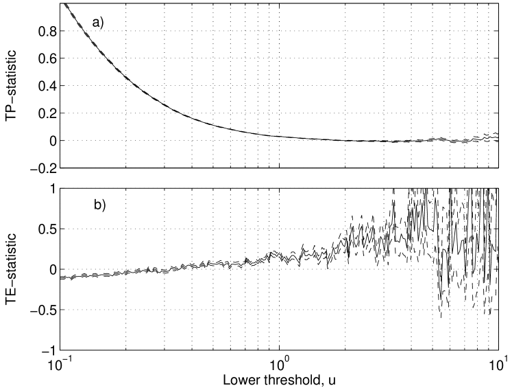
Figure 2: (a) TP-statistic and (b) TE-statistic as function of the lower cut-off $u$ for positive returns of the NSE with time interval $\Delta t$ = 1 min. The broken lines indicate plus or minus one standard deviation of the statistics.

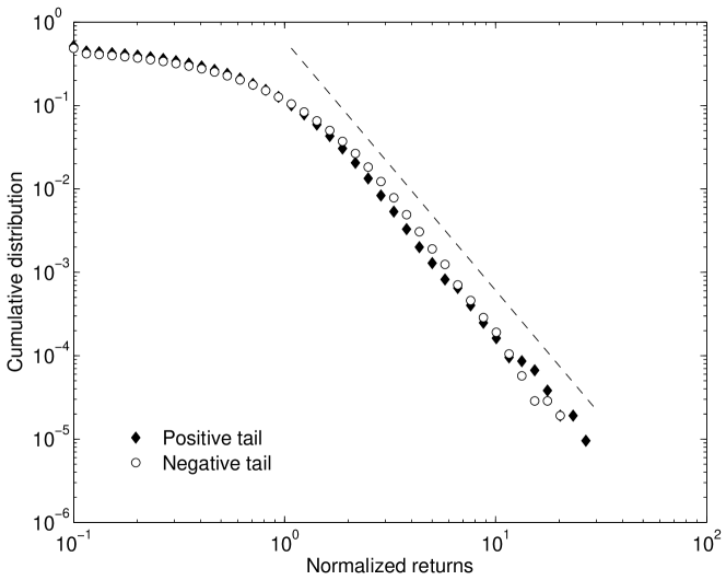
Figure 3: The cumulative distribution of the normalized 1-min return for the NSE Nifty index. The broken line indicates a power-law with exponent $\alpha=3$.

Fig. 2 shows visually the deviation of the empirical data from the power-law and exponential distributions. The TP- and the TE-statistics are plotted as functions of the lower cut-off $u$ for 1-min returns of the NSE Nifty index. The TP-statistic shows a large deviation till $u\leq 1$, after which it converges to zero indicating power-law behavior for large $u$. Correspondingly, the TE-statistic excludes an exponential model for $u\geq 1$ as well as for very low values of $u$, although over the intermediate range $2\times 10^{-1}<u<6\times 10^{-1}$ an exponential approximation may be possible.

Fig. 3 shows the cumulative distribution of the normalized returns for $\Delta t=1$ min. For both positive and negative tails, there is an asymptotic power-law behavior. The power-law regression fit for the region $r\geq 2$ give exponents for the positive and the negative tails estimated as

$$\alpha=\left\{\begin{array}[]{ll}2.98\pm 0.09&\mbox{(positive tail)}\\ 3.37\pm 0.10&\mbox{(negative tail).}\end{array}\right.$$ (5)

Note that, to avoid artifacts due to data measurement process in the calculation of return distribution for $\Delta t<1$ day, we have removed the returns corresponding to overnight changes in the index value.

We also perform an alternative estimation of the tail index of the the above distribution by using the Hill estimator Hill (1975), which is the maximum likelihood estimator of $\alpha$. For finite samples, however, the expected value of the Hill estimator is biased and depends crucially on the choice of the number of order statistics used for calculation. We have used the bootstrap procedure Pictet et al. (1998) to reduce this bias and to choose the optimal number of order statistics for calculating the Hill estimator, described in detail in the Appendix B. We found $\alpha\simeq$ 3.22 and 3.47 for the positive and the negative tails, respectively.

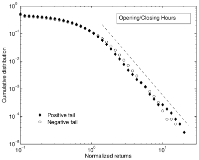
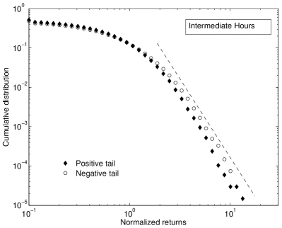
Figure 4: Intra-day variation in the cumulative distribution of the normalized 1-min return for the NSE Nifty index: return distribution during (left) the opening and closing hours (the broken line indicates a power law with exponent $\alpha=3$) and (right) the intermediate time period (the broken line indicates a power law with exponent $\alpha=4$).

To investigate the effect of intra-day variations in market activity, we analyze the 1-min return time series by dividing it into two parts, one corresponding to returns generated in the opening and the closing hours of the market, and the other corresponding to the intermediate time period. In general, it is known that the average intra-day volatility of stock returns follows an U-shaped pattern Wood et al. (1985); Harris (1986) and one can expect this to be reflected in the nature of the fluctuation distribution for the opening and closing periods, as opposed to the intervening period. We indeed find the index fluctuations for these two data sets to be different (Fig. 4). In particular, the cumulative distribution tail for the opening and closing hour returns show a power-law scaling with exponent close to $3$, whereas for the intermediate period we see that the exponent is close to $4$. This observation is similar to that reported for the German DAX index, where removal of the first few minutes of return data after the daily opening resulted in a power-law distribution with a different exponent compared to the intact data set Lux (2001).

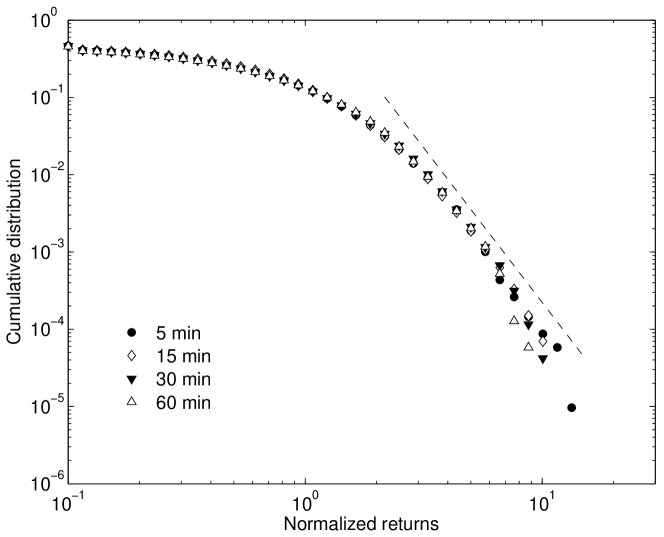
Figure 5: The negative tail of the cumulative distribution of the NSE Nifty index returns for different time intervals $\Delta t$ upto $60$ min. The broken line indicates a power-law with exponent $\alpha=4$.

Next, we extend our analysis for longer time scales, $\Delta t$. We find that time aggregation of the data increases the $\alpha$ value. The tail of the return distribution still retains its power-law form (Fig. 5), until at longer time scales the distribution slowly converges to Gaussian behavior (Table 1). The results are invariant with respect to whether one calculates return using the sampled index value at the end point of an interval or the average index value over the interval. Figure 5 shows the cumulative distribution of normalized Nifty returns for time scales up to 60 min. However, using a similar procedure for generating daily returns from the tick-by-tick data would give us a very short time series. This is not enough for reliable analysis as it takes at least 3000 data points for a meaningful estimate of the tail index.

Table 1: Comparison of the power-law exponent $\alpha$ of the cumulative distribution function for various index returns. Power-law regression fits are done in the region $r\geq 2$. The Hill estimator is calculated using the bootstrap algorithm.

Index	$\Delta t$	Power-law fit		Hill estimator
		Positive	Negative	Positive	Negative
Nifty (’03-’04)	1 min	$2.98\pm 0.09$	$3.37\pm 0.10$	$3.22\pm 0.03$	$3.47\pm 0.03$
	5 min	$4.42\pm 0.37$	$3.44\pm 0.21$	$4.51\pm 0.03$	$4.84\pm 0.03$
	15 min	$5.58\pm 0.88$	$3.96\pm 0.27$	$6.25\pm 0.03$	$4.13\pm 0.04$
	30 min	$5.13\pm 0.41$	$3.92\pm 0.45$	$5.65\pm 0.03$	$4.30\pm 0.03$
	60 min	$5.99\pm 1.52$	$4.42\pm 0.65$	$7.85\pm 0.03$	$5.11\pm 0.04$
Nifty (’90-’06)	1 day	$3.10\pm 0.34$	$3.18\pm 0.28$	$3.33\pm 0.14$	$3.37\pm 0.14$
Sensex (’91-’06)	1 day	$3.33\pm 0.77$	$3.45\pm 0.25$	$2.93\pm 0.15$	$3.84\pm 0.12$

For this reason, we have analyzed the daily data using a different source, with the time period stretching over a considerably longer period (16 years). The return distribution of the daily closing data of Nifty shows qualitatively similar behavior to the 1 min distribution. The Sensex index, which is from another stock exchange, also follows a similar distribution(Fig. 6). The measured exponent values are all close to 3. This does not contradict the earlier observation that $\alpha$ increases with $\Delta t$, because, increasing the sample size (as has been done for $\Delta t=1$ day) improves the estimation of $\alpha$. This underlines the invariance of the nature of market fluctuations with respect to time aggregation, interval used and different exchanges.

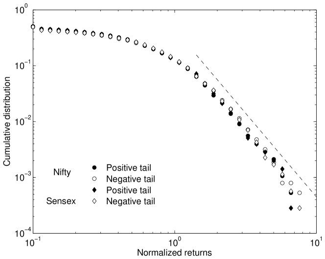
Figure 6: The cumulative distribution of the normalized 1-day return for the NSE Nifty and BSE Sensex index. The broken line indicates a power-law with exponent $\alpha=3$.

IV Discussion and Conclusion

The much shorter data-set of the BSE 500 daily returns shows a significant departure from power-law behavior, essentially following an exponential distribution (Figure not shown). This is not surprising, as looking at data over shorter periods can result in misidentification of the nature of the distribution. Specifically, the relatively low number of data points corresponding to returns of large magnitude can lead to missing out the long tail. In fact, even for individual stocks in developed markets, although the tails follow a power-law, the bulk of the return distribution is exponential Silva et al. (2004). This problem arising from using limited data-sets might be one of the reasons why some studies have seen significant deviation of index return distribution from a power-law.

A more serious problem is that the analysis in many of these studies is usually performed only by graphically fitting the data with a theoretical distribution function. Such a visual judgement of the goodness of fit may lead to erroneous characterization of the nature of fluctuation distribution. Graphical procedures are often subjective, particularly with respect to the choice of the lower cut-off upto which fitting is carried out. This dependence of the theoretical distribution that best describes the tail on the cut-off, has been explicitly demonstrated through the use of TP- and TE-statistic in this paper. Moreover, recent studies have criticized the reliability of graphical methods by showing that least square fitting for estimating the power-law exponent tends to provide biased estimates, while the maximum likelihood method produces more accurate and robust estimates Goldstein et al. (2004); Coronel-Brizio and Hernandez-Montoya (2005b). So we have used the Hill estimator to determine the tail exponents.

If the individual stocks follow the inverse cubic law, it would be reasonable to suppose that the index, which is a weighted average of several stocks, will also behave similarly, provided the different stocks move in a correlated fashion Gopikrishnan et al. (1999). As the price movements of stocks in an emerging market are even more correlated than in developed markets Pan and Sinha (2007b), it is expected that the returns for stock prices and the index should follow the same distribution. Therefore, the demonstration of the inverse cubic law for the index fluctuations in the Indian market is consistent with our previous study Pan and Sinha (2007a) showing that the individual stock prices in this market follow the same behavior.

On the whole, our study points out the remarkable robustness of the nature of the fluctuation distribution for Indian market indices. While, in the period under study, the NSE had begun operation and rapidly increased in terms of activity, the BSE had existed for a long time prior to this period and showed a significant decrease in market share. However, both showed very similar fluctuation behavior. This indicates that, at least in the Indian context, the distribution of returns is invariant with respect to markets. The fact that the distribution is quantitatively same as developed markets, implies that it is also probably independent of the state of the economy. In addition, our observation that the intra-day return distribution of Indian market index show properties similar to that reported for developed markets, suggest that even at this level of detail the fluctuation behavior of the two kinds of markets are rather similar. Therefore, our results indicate that although markets may differ from each other in terms of (i) the details of their components, (ii) the nature of interactions and (iii) their susceptibility to news from outside the market, there may be universal mechanisms responsible for generating market fluctuations as indicated by the observation of invariant properties. The rigorous demonstration of such a universal law for market behavior is significant for the physics of strongly interacting complex systems, as it suggests the existence of robust features that are independent of individual details of different systems.

Appendix A TP-statistic and TE-statistic

A.1 TP-statistic

Consider the power-law distribution,

$$F(x)=1-P_{c}(x)=1-(u/x)^{\alpha},~{}{\rm for}~{}x\geq u,$$ (6)

where $u$ is the lower cut-off, and $\alpha$ is the power-law exponent for the distribution. For a finite sample $x_{1},\dots,x_{n}$, the TP-statistic, TP($x_{1},\dots,x_{n}$), is defined such that it converges to zero asymptotically for large $n$ Pisarenko and Sornette (2006); Pisarenko et al. (2004). If the underlying distribution for a sample differs from the power-law form given in Eq.(6), TP is seen to deviate from zero. This statistic is based on the first two normalized statistical log-moments of the power-law distribution,

$$E_{1}=E\left[\log\frac{X}{u}\right]=\int_{u}^{\infty}\log\frac{x}{u}dF(x)=\frac{1}{\alpha},~{}{\rm and}$$ (7)

$$E_{2}=E\left[\log^{2}\frac{X}{u}\right]=\int_{u}^{\infty}\log^{2}\frac{x}{u}dF(x)=\frac{2}{\alpha^{2}},$$ (8)

where, $E[z]$ represents the mathematical expectation of $z$. The TP-statistic is then defined as

$$\mathrm{TP}=\left[\frac{1}{n}\sum_{k=1}^{n}\log\frac{x_{k}}{u}\right]^{2}-\frac{1}{2n}\sum_{k=1}^{n}\log^{2}\frac{x_{k}}{u},$$ (9)

which tends to zero as $n\rightarrow\infty$. The estimation of the standard deviation for the TP statistic is provided by the standard deviation of the sum

$$\left(\frac{E_{2}}{2}-2E_{1}^{2}\right)+\frac{1}{n}\sum_{k=1}^{n}\left[2E_{1}\log\frac{x_{k}}{u}-\frac{1}{2}\log^{2}\frac{x_{k}}{u}\right].$$ (10)

A.2 TE-Statistics

Consider the exponential distribution,

$$F(x)=1-P_{c}(x)=1-\exp(-(x-u)/d),~{}{\rm for}~{}x\geq u,$$ (11)

where $u$ is the lower cut-off, and $d(>0)$ is the scale parameter of the distribution. For a finite sample $x_{1},\dots,x_{n}$, the TE statistic, TE($x_{1},\dots,x_{n}$), is defined such that it converges to zero asymptotically for large $n$ Pisarenko and Sornette (2006). If the underlying distribution for a sample differs from the exponential form given in Eq.(11), TE is seen to deviate from zero. This statistic is based on the first two normalized statistical (shifted) log-moments of the exponential distribution,

$$E_{1} = E\left[\log\left(\frac{X}{u}-1\right)\right]=\int_{u}^{\infty}\log\left(\frac{x}{u}-1\right)dF(x)$$ (12)

$$= \log\frac{d}{u}-\gamma,$$

where $\gamma=0.577215$ is the Euler constant, and

$$E_{2} = E\left[\log^{2}\left(\frac{X}{u}-1\right)\right]=\int_{u}^{\infty}\log^{2}\left(\frac{x}{u}-1\right)dF(x)$$ (13)

$$= \left(\log\frac{d}{u}-\gamma\right)^{2}+\frac{\pi^{2}}{6}.$$

As before, $E[\dots]$ denotes the mathematical expectation. The TE-statistic is then defined as

$$\mathrm{TE}=\frac{1}{n}\sum_{k=1}^{n}\log^{2}\left(\frac{x_{k}}{u}-1\right)-\left[\frac{1}{n}\sum_{k=1}^{n}\log\left(\frac{x_{k}}{u}-1\right)\right]^{2}-\frac{\pi^{2}}{6},$$ (14)

which tends to zero as $n\rightarrow\infty$. The estimation of the standard deviation for the TE-statistic is provided by the standard deviation of the sum

$$\frac{1}{n}\sum_{k=1}^{n}\left[\log\left(\frac{x_{k}}{u}-1\right)-E_{1}\right]^{2}.$$ (15)

Appendix B Hill estimation of the tail exponent $\alpha$

The Hill estimator gives consistent estimate of the tail exponent $\alpha$ from random samples of a distribution with an asymptotic power-law form. For our analysis, we arrange the returns in decreasing order such that $r_{1}>\cdots>r_{n}$. Then the Hill estimator (based on the largest $k+1$ values) is given as

$$\gamma_{k,n}=\frac{1}{k}\sum_{i=1}^{k}{\log\frac{r_{i}}{r_{k+1}}},$$ (16)

for $k=1,\cdots,n-1$. The estimator $\gamma_{k,n}\rightarrow\alpha^{-1}$ when $k\rightarrow\infty$ and $k/n\rightarrow 0$. However, for a finite time series, the expectation value of the Hill estimator is biased, i.e., it will consistently over or underestimate $\alpha$. Further, $\gamma$ depends critically on our choice of $k$, the order statistics used to compute the Hill estimator.

If the form of the distribution function from which the random sample is chosen is known, then the bias and the stochastic error variance of the Hill estimator can be calculated. From this, the optimum $k$ value can be obtained such that the asymptotic mean square error of the Hill estimator is minimized. Increasing $k$ reduces the variance because more data are used, but increases the bias because the power-law is assumed to hold only in the extreme tail. Unfortunately, the distribution for the empirical data is not known and hence this procedure has to be replaced by an asymptotically equivalent data driven process.

One such method is subsample bootstrap method. This method can be used to estimate an optimal number for the order statistics ($\bar{k}$) that will reduce the asymptotic mean square error of the Hill estimator. However, this process requires the choice of certain parameters, e.g., the subsample size $n_{s}$ and the range of $k$ values in which one searches for the minimum of the bootstrap statistics. We briefly describe this procedure below; for details and mathematical validation of this procedure, please see Ref. Pictet et al. (1998).

We assume the underlying empirical distribution function to be heavy-tailed, viz.,

$$P_{c}(x)=ax^{-\alpha}[1+bx^{-\beta}+o(x^{-\beta})],$$ (17)

with $\alpha,\beta,a>0$ and $-\infty<b<\infty$. We first calculate an initial $\gamma_{0}=\gamma_{k_{0},n}$ for the original series with a reasonably chosen (but non-optimal) $k_{0}$. Then we choose various subsamples of size $n_{s}$ randomly from the original series, which are orders of magnitude smaller then $n$. The quantity $\gamma_{0}$ is a good approximation of subsample $\alpha^{-1}$, since the error in $\gamma$ is much larger for $n_{s}$ than for $n$ observations. The optimal order statistics $\bar{k}_{s}$ for the subsample is found by computing $\gamma(k_{s},n_{s})$ for different values of $k_{s}$ and then minimising the deviation from $\gamma_{0}$. Given $\bar{k}_{s}$, the suitable full sample $\bar{k}$ can be found by using

$$\bar{k}=\bar{k}_{s}\left(\frac{n}{n_{s}}\right)^{\frac{2\beta}{2\beta+\alpha}}.$$ (18)

Here the initial estimate of $\alpha$ is taken to be $1/\gamma_{0}$. Further, we have considered $\beta=\alpha$, as done by Hall Hall (1990), although the results are not very sensitive to the choice of $\beta$. Once $\bar{k}$ is calculated, the final estimate of the tail index is given by $\alpha=1/\gamma_{\bar{k},n}$.

For calculating the initial $\gamma_{0}$ we have chosen $k_{0}$ to be $0.5\%$ of the sample size $n$. 1000 subsamples, each of size $n_{s}=n/40$, are randomly picked from the full data set. To obtain optimal $k_{s}$, we confine ourselves to $4\%$ of the subsample size $n_{s}$. To find the stochastic error in our estimation of $\alpha$, we have computed the 95% confidence interval as given by $\pm 1.96[1/(\alpha^{2}m)]^{1/2}$. Although a Jackknife algorithm can also be used to calculate this error bound, the results obtained using this method will be close to that obtained using the bootstrap method over many realizations Pictet et al. (1998), as we have done in this paper.

References

- Mantegna and Stanley (1999) R. N. Mantegna and H. E. Stanley, Introduction to Econophysics (Cambridge University Press, Cambridge, 1999).
- Bouchaud and Potters (2003) J. P. Bouchaud and M. Potters, Theory of Financial Risk and Derivative Pricing (Cambridge University Press, Cambridge, 2003), 2nd ed.
- Chatterjee and Chakrabarti (2006) A. Chatterjee and B. K. Chakrabarti, eds., Econophysics of Stock and Other Markets (Springer, Milan, 2006).
- Bachelier (1900) L. Bachelier, Annales Scientifiques de l’École Normale Supérieure Sér 3, 21 (1900).
- Osborne (1964) M. Osborne, in The Random Character of Stock Market Prices (MIT Press, Cambridge, MA, 1964), pp. 100–128.
- Fama (1965) E. F. Fama, Journal of Business 38, 34 (1965).
- Mandelbrot (1963) B. Mandelbrot, Journal of Business 36, 394 (1963).
- Mantegna and Stanley (1995) R. N. Mantegna and H. E. Stanley, Nature 376, 46 (1995).
- Gopikrishnan et al. (1998) P. Gopikrishnan, M. Meyer, L. A. Nunes Amaral, and H. E. Stanley, Eur. Phys. Jour. B 3, 139 (1998).
- Gopikrishnan et al. (1999) P. Gopikrishnan, V. Plerou, L. A. Nunes Amaral, M. Meyer, and H. E. Stanley, Phys. Rev. E 60, 5305 (1999).
- Lux (1996) T. Lux, Applied Financial Economics 6, 463 (1996).
- Lux and Marchesi (1999) T. Lux and M. Marchesi, Nature 397, 498 (1999).
- Chowdhury and Stauffer (2004) D. Chowdhury and D. Stauffer, Eur. Phys. Jour. B 8, 477 (2004).
- Bornholdt (2001) S. Bornholdt, Int. J. Mod. Phys. C 12, 667 (2001).
- Iori (2002) G. Iori, Journal of Economic Behavior & Organization 49, 269 (2002).
- Sinha (2006) S. Sinha, in Ref [3] , pp. 159–162.
- Mandelbrot (1997) B. B. Mandelbrot, Fractals and Scaling in Finance (Springer, New York, 1997).
- Bacry et al. (2001) E. Bacry, J. Delour, and J. F. Muzy, Phys. Rev. E 64, 026103 (2001).
- Bouchaud (2005) J. P. Bouchaud, Chaos 15, 026104 (2005).
- Storer and Gunner (2002) R. Storer and S. M. Gunner, Int. J. Mod. Phys. C 13, 893 (2002).
- Wang and Hui (2001) B. Wang and P. Hui, Eur. Phys. Jour. B 20, 573 (2001).
- Kaizoji and Kaizoji (2003) T. Kaizoji and M. Kaizoji, Advances in Complex Systems 6, 303 (2003).
- Oh et al. (2006) G. Oh, C.-J. Um, and S. Kim, physics/0601126 (2006).
- Yang et al. (2006) J.-S. Yang, S. Chae, W.-S. Jung, and H.-T. Moon, Physica A 363, 377 (2006).
- Miranda and Riera (2001) L. C. Miranda and R. Riera, Physica A 297, 509 (2001).
- Gleria et al. (2002) I. Gleria, R. Matsushita, and S. D. Silva, Economics Bulletin 7, 1 (2002).
- Coronel-Brizio and Hernandez-Montoya (2005a) H. F. Coronel-Brizio and A. R. Hernandez-Montoya, Revista Mexicana de Fisica 51, 27 (2005a).
- Rak et al. (2007) R. Rak, S. Drozdz, and J. Kwapien, Physica A 374, 315 (2007).
- Jondeau and Rockinger (2003) E. Jondeau and M. Rockinger, Journal of Empirical Finance 10, 559 (2003).
- Matia et al. (2004) K. Matia, M. Pal, H. Salunkay, and H. E. Stanley, Europhys. Lett. 66, 909 (2004).
- Plerou et al. (1999) V. Plerou, P. Gopikrishnan, L. A. Nunes Amaral, M. Meyer, and H. E. Stanley, Phys. Rev. E 60, 6519 (1999).
- Pan and Sinha (2007a) R. K. Pan and S. Sinha, Europhys. Lett. 77, 58004 (2007a).
- Sarma (2005) M. Sarma, Report 2005-003, Eurandom, (2005).
- ARS (2006) Tech. Rep., World Fedration of Exchanges (2006).
- Sinha and Pan (2006) S. Sinha and R. K. Pan, in Ref [3] , pp. 24–34.
- Pisarenko and Sornette (2006) V. Pisarenko and D. Sornette, Physica A 366, 387 (2006).
- Pisarenko et al. (2004) V. Pisarenko, D. Sornette, and M. Rodkin, Computational Seismology 35, 138 (2004).
- Hill (1975) B. M. Hill, Annals of Statistics 3, 1163 (1975).
- Pictet et al. (1998) O. V. Pictet, M. M. Dacorogna, and U. A. Muller, in A Practical Guide to Heavy Tails (Birkhauser, 1998), pp. 283–310.
- Wood et al. (1985) R. A. Wood, T. H. McInish, and J. K. Ord, Journal of Finance 40, 723 (1985).
- Harris (1986) L. Harris, Journal of Financial Economics 16, 99 (1986).
- Lux (2001) T. Lux, Applied Financial Economics 11, 299 (2001).
- Silva et al. (2004) A. C. Silva, R. E. Prange, and V. M. Yakovenko, Physica A 344, 227 (2004).
- Goldstein et al. (2004) M. L. Goldstein, S. A. Morris, and G. G. Yen, Eur. Phys. Jour. B 41, 255 (2004).
- Coronel-Brizio and Hernandez-Montoya (2005b) H. Coronel-Brizio and A. Hernandez-Montoya, Physica A 354, 437 (2005b).
- Pan and Sinha (2007b) R. K. Pan and S. Sinha, Phys. Rev. E 76, 046116 (2007).
- Hall (1990) P. Hall, Journal of Multivariate Analysis 32, 177 (1990).