Fast Computation of Voigt Functions via Fourier Transforms

Abstract

This work presents a method of computing Voigt functions and their derivatives, to high accuracy, on a uniform grid. It is based on an adaptation of Fourier-transform based convolution. The relative error of the result decreases as the fourth power of the computational effort. Because of its use of highly vectorizable operations for its core, it can be implemented very efficiently in scripting language environments which provide fast vector libraries. The availability of the derivatives makes it suitable as a function generator for non-linear fitting procedures.

Introduction

The computation of Voigt line profiles is an issue which has been dealt with over a long time in the literature [1, 2, 3, 4, e.g.]. Nonetheless, it remains a computationally interesting problem because it is still fairly expensive to compute profiles to high accuracy. This paper presents a method which is fast and very simple to implement. It is similar to the method of [3], but capable of much higher precision for a given computational effort. More importantly, the method described here computes not only the Voigt function itself, but its derivatives with respect to both the Gaussian and Lorentzian widths, which are helpful for non-linear curve fitting.

Because the method is based on Fourier transforms, and generates a grid of values for the function in a single operation, it is particularly suitable for (but not restricted to) use in scripting environments, where Fast Fourier Transforms (FFTs) and other vector operations are available as part of the language library, and execute at very high speed. Thus, in Matlab®, Python (with Numeric or numpy), Mathematica®, Octave, and other similar environments, it may find particular applicability. Such environments provide a trade-off of speed for flexibility, and this method allows one to take a much smaller speed penalty than would be exacted using other algorithms implemented in the scripting language.

A method such as this one, which contains no inherent approximations, has advantages over other approximate methods in that it can be adapted very easily to the desired level of precision of the task at hand. Selecting the density of the computational grid and the length into the tails to which the computation is carried out sets the accuracy. The grid density does not affect the accuracy of the values this produces directly, but does affect the accuracy to which interpolation may be carried out between the computed points. The distance into the tails to which the profile is computed does affect the accuracy of the step (defined below) which corrects for periodic boundary conditions, and it converges as the fourth power of this distance.

As an aside on notation, most papers working with the Voigt function historically have defined it in terms of a single parameter, the ratio of the Lorentzian to Gaussian width. This work, presents the results in a slightly different form, which is more useful for direct computation. The equations below are computed in terms of the Lorentzian width (which I call $\alpha$) and the standard deviation of the Gaussian distribution $\sigma$. The parameter $y$ in Drayson [1] is $\alpha/(\sqrt{2}\sigma)$ in my notation. In this form, the transforms produce functions fully scaled and ready for direct interpolation.

Theory

The Voigt function is a convolution of a Lorentzian profile and a Gaussian,

$$V(\alpha,\sigma;\,x)\propto\int_{-\infty}^{\infty}\frac{e^{-t^{2}/2\sigma^{2}}}{(x-t)^{2}+\alpha^{2}}\,dt$$ (1)

and can be easily written down in Fourier transform space using the convolution theorem:

$$\tilde{V}(\alpha,\sigma;\,k)=\exp\left[-\sigma^{2}k^{2}/2-\alpha\left|k\right|\right]$$ (2)

Also, of great importance to using this in fitting procedures, the derivatives of this function with respect to its parameters can be computed:

$$\frac{\partial\tilde{V}}{\partial\alpha}=-\left|k\right|\tilde{V}$$ (3)

and

$$\frac{\partial\tilde{V}}{\partial\sigma}=-\sigma k^{2}\tilde{V}$$ (4)

and since the differentiation in these cases commutes with the transform, these are the transforms of the appropriate derivatives of the function itself.

Note that, since this transform method generates functions with a fixed area, these are the derivatives with respect to the widths at fixed area, rather than at fixed amplitude. This implies that fitting carried out using functions computed this way is most appropriately done using $\alpha$, $\sigma$, and area as parameters.

This result is exactly correct in the full Fourier transform space. For practical computation, though, one wishes to reduce this into something which is computed rapidly on a discrete lattice using Fast Fourier Transform (FFT) techniques, and then interpolated between the lattice points. The difference between the full continuous transform and the discrete transform is, of course, that the function produced by a discrete transform is periodic. In effect, by discretely sampling the series in Fourier space, one is computing, instead of the exact convolution, a closely related function which has had periodic boundary conditions applied. This affects the shape of the tails of the distribution, but in a way which is fairly easily fixed.

First, when doing the discrete transforms, it is necessary to decide how far out in $k$-space it is necessary to have data. In general, one wants to assure the function is nicely band-limited, which means no significant power exists at the highest $k$. Practically speaking, setting the argument of the exponential in eq. 2 to something like –25 at the boundary means the highest frequency component is $e^{-25}$ or about $10^{-11}$ of the DC component. To achieve this, define the absolute value of the log of the tolerance to be $\gamma$ (25 for the example here) and solve $\sigma^{2}k^{2}/2+\alpha\left|k\right|=\gamma$. This is a simple quadratic equation, but because one doesn’t know in advance how dominant the relative terms are, one should solve it with a bit of care. The stable quadratic solution presented in Numerical Recipes [5] can be adapted to be

$$k_{max}=\frac{2\gamma}{\alpha+\sqrt{\alpha^{2}+2\gamma\sigma^{2}}}$$ (5)

This is simpler than the full solution in [5] since the signs of both $\alpha$ and $\sigma$ are known in advance.

Now, note that the periodic solution is really an infinite comb of functions shaped like the desired one, added together. Since, beyond a few $\sigma$ from the center, the function is close to Lorentzian, one has really computed the desired function plus an infinite series of offset simple Lorentzians:

$$V(\alpha,\sigma;\,x)=V_{act}(\alpha,\sigma;\,x)+\frac{\alpha}{\pi}\sum_{n\neq 0}\frac{1}{(x-n\Delta)^{2}+\alpha^{2}}$$ (6)

where $\Delta$ is the period of the function. However, the infinite sum can be computed analytically. It is:

$$\epsilon\equiv\frac{\alpha}{\pi}\sum_{n\neq 0}\frac{1}{(x-n\Delta)^{2}+\alpha^{2}}=\frac{\sinh\frac{2\pi\alpha}{\Delta}}{\Delta\left(\cosh\frac{2\pi\alpha}{\Delta}-\cos\frac{2\pi x}{\Delta}\right)}-\left(\frac{\alpha}{\pi}\right)\frac{1}{x^{2}+\alpha^{2}}$$ (7)

$$\frac{\partial\epsilon}{\partial\alpha}=\frac{\left(\alpha^{2}-x^{2}\right)}{\pi\left(\alpha^{2}+x^{2}\right)^{2}}+\frac{2\pi\cosh\left(\frac{2\alpha\pi}{\Delta}\right)}{\Delta^{2}\left(\cosh\frac{2\pi\alpha}{\Delta}-\cos\frac{2\pi x}{\Delta}\right)}-\frac{2\pi\sinh^{2}\left(\frac{2\alpha\pi}{\Delta}\right)}{\Delta^{2}\left(\cosh\frac{2\pi\alpha}{\Delta}-\cos\frac{2\pi x}{\Delta}\right)^{2}}$$ (8)

Since the derivative with respect to $\sigma$ is very localized, and falls to zero rapidly at the boundaries, no correction is needed for it.

Although these equations look computationally intensive, they are not so at all. Note that the $\cosh$ and $\sinh$ terms are of a constant, and not evaluated at each point. Also, for the usual Fourier-space case, $\Delta=2x_{max}$ so the $\cos$ term is just an evaluation of the cosine from $-\pi$ to $\pi$ on the same grid the rest of the function will be evaluated. If the Voigt function is to be evaluated for many different $\alpha,\,\sigma$ pairs (as is the case in fitting routines), but always on a grid with a fixed number of points, this cosine only gets evaluated once, too, and can be cached for reuse. Also, the correction and its derivative with respect to $\alpha$ share most of their terms in common, so this correction is really a simple algebraic adjustment to the raw function table.

The correction term in eq. 7 is an approximation based on all the other nearby peaks being entirely Lorentzian, and works well. However, it can be improved by a scaling argument, which works significantly better. The non-Lorentzian nature of the correction is due to the convolution of the Gaussian with the curvature of the Lorentzian causing a slight widening even on the tails. Note that convolution of a function with a Gaussian only affects even derivatives (by symmetry), so the second derivative term is the lowest order this could affect. Also note that this effect is getting bigger as one approaches the next peak over (the edge of the boundary). Thus, one can try a correction of multiplying the right hand side of eq. 7 by $1+ax^{2}$ where $a$ is to be determined. Much of the structure of $a$ can be obtained by scaling, and it should be $a\propto\sigma^{2}/\Delta^{4}$. Empirical testing has shown that a constant of 32 appears optimal, so an improvement on eq. 7 is:

$$\epsilon=\left[\frac{\sinh\frac{2\pi\alpha}{\Delta}}{\Delta\left(\cosh\frac{2\pi\alpha}{\Delta}-\cos\frac{2\pi x}{\Delta}\right)}-\left(\frac{\alpha}{\pi}\right)\frac{1}{x^{2}+\alpha^{2}}\right]\left(1+\frac{32\sigma^{2}x^{2}}{\Delta^{4}}\right)$$ (9)

This improves the original correction by almost an order of magnitude in the peak error at the bounds of the interval, and the RMS error is reduced by about a factor of 5 for most test cases.

Note that this expression also provides an error estimate for the calculation, which can be used to determine an appropriate value for $\Delta$. Assuming the error is of the same order as the final correction term, which should be conservative, one can proceed to evaluate it at the boundary of the interval, where $x=\Delta/2$, and evaluating eq. 7 assuming $\Delta\gg\alpha$, the error estimate is then

relative  err $$\sim \textrm{(small\, coefficient)}\times 2\,\sigma^{2}/\Delta^{2}$$ (10)

Note that, although this is $\propto 1/\Delta^{2}$, this is the relative error. The function itself is decreasing at the boundary as $1/\Delta^{2}$ so the absolute error scales with $1/\Delta^{4}$, as expected.

The road not taken

There is another way one could consider carrying out this computation, which looks elegant and easy from the outset, but actually is computationally much more expensive. I will outline it here as a warning to others.

Instead of fixing the periodicity error by adding on the correction of eq. 7 or eq. 9, one might be tempted to fix the problem in advance, before the transforms are carried out from $k$-space to real space. The obvious solution is to try to compute the transform of the difference between the Voigt function and a pure Lorentzian, and then add the pure Lorentzian back in afterward, not as an infinite sum as in the correction equations, but just as a single copy. One would compute

$$\tilde{V}_{0}(\alpha,\sigma;\,k)=\left(\exp\left[-\sigma^{2}k^{2}/2\right]-1\right)\exp\left[-\alpha\left|k\right|\right]$$ (11)

and then transform this, and add back on the Lorentzian which was subtracted. This turns out to be computationally very inefficient, though. When computing the transforms, one wants a cleanly band-limited function in $k$-space, with the power in the highest frequency channels vanishing rapidly. In the case of eq. 2, this is clearly the case, since the $-\sigma^{2}k^{2}/2$ term makes the exponential disappear relatively rapidly even for fairly modest values of $\sigma$ and $k$. In the case of eq. 11, though, $\tilde{V}_{0}$ only vanishes as fast as the $\exp\left[-\alpha\left|k\right|\right]$ term, which falls off much more slowly. Thus, one has to carry out the transforms to much higher values of $k$ to get convergence. This turns out practically to be a huge penalty. Even in the case of $\sigma\approx k$, it requires about a few times more terms, and in the case $\sigma\gg k$, it is much worse, since the extremely rapid falloff of the Gaussian in $k$-space allows one to sample only quite small values of $k$ to get very good performance.

Application

The most probable way the author sees these gridded functions being used is to load cubic spline interpolation tables to generate values at points which may not lie on the grid. This way, one can compute the Fourier transforms on grids of sizes convenient for FFT algorithms (often, powers of two, but using. e.g. FFTW [6], many other grid sizes can be conveniently transformed), and then use the interpolator to fill in the values desired. Because of both the shape of these functions and the wide dynamic range they typically encompass, it is likely that it will be useful to interpolate the logarithm of the function. Especially if $\sigma\gg\alpha$, so the center looks Gaussian, log interpolation is extremely beneficial, since the logarithm of the Gaussian part is just parabolic, and exactly interpolable by a cubic spline interpolator.

In fitting work, one more derivative is needed than the ones computed in eqs. 3 and 4, which is the derivative with respect to the coordinate itself, which is needed to solve for the center of a peak. Although this could easily be computed in Fourier transform space by inverse transforming $i\,k\,\tilde{V}(k)$, it also falls directly out of the cubic spline interpolation. The value of a splined function at a point is computed (see the discussion of splining in [5] for notation) as

$$h = x_{1}-x_{0}$$

$$a = \frac{x_{1}-x}{h}$$

$$b = 1-a$$

$$y = a\,y_{0}+b\,y_{1}+\frac{h^{2}}{6}\left[(a^{3}-a)\,y_{0}^{\prime\prime}+(b^{3}-b)\,y_{1}^{\prime\prime}\right]$$ (12)

then the first derivative is

$$y^{\prime}=\frac{y_{1}-y_{0}}{h}+\frac{h}{6}\left[(3\,b^{2}-1)\,y_{1}^{\prime\prime}-(3\,a^{2}-1)\,y_{0}^{\prime\prime}\right]$$ (13)

This is the method preferred by the author of this work for this derivative.

Error Analysis

Figure 1 shows sample functions computed by this method, and the relative errors associated with this computation. These were computed using the extra error correction of eq. 9. The scaling of the errors is fairly easy to compute from the underlying equations. In general, the errors scale as $\Delta^{-4}$ when $\sigma$ and $\alpha$ are held constant. For most practical applications, it is likely that the need to compute the tails far enough from the center that the entire spectrum is covered by the calculation results in the tails being calculated sufficiently far out that the accuracy is not a concern. In Figure 1, the curve (5) shows the result when $\Delta=80\sigma$ (tails computed to $40\sigma)$, and even in this case the peak relative error is $10^{-4}$ (in a part of the curve off the graph). Most practical cases are likely to need the tails much farther out than this, resulting in the accuracy automatically being better than this. As an example, though, of pushing the computation to very narrow tails, the curve (4) shows the results for the tails being computed to only $10\sigma$. Even in this case, the relative error only exceeds $10^{-3}$ at the very edge of the domain.

Note that these are computed with $\alpha=1$ and $\sigma$ being varied. Since the shape of the Voigt function really only depends on $\alpha/\sigma$ (related to the usual $y$ parameter), this completely specifies the shape of the function except for an overall width scale. Also, note that the cases shown are all for $\sigma\geq\alpha;$ the case of small $\sigma$ is a limiting case, and the errors look much as they do for $\sigma=\alpha$.

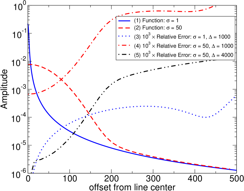
Figure 1: Plot of Voigt Functions with $\alpha=1$ evaluated by this method, and the relative errors (as computed by adaptive numerical integration of the convolution at each point).

Conclusion

Because of relatively slow convergence, simple FFT-based convolution has not fared well in the Voigt-function computation arena. Nonetheless, this method has always had an advantage in simplicity and vectorizability. Also, it is trivial to get the derivatives of the Voigt function with respect to its width parameters from transform-based methods. This makes this algorithm most useful for cases in which line strengths, widths, and positions are all variable. The convergence enhancement can also be easily extended to line shapes in which a non-Gaussian function is convolved with a Lorentzian.

By combining the traditional transform-based method with a convergence-enhancing operation, the result is a method which is fast, accurate, and extremely easy to implement. It should find particular application for fitting work carried out in many widely used scripting languages, in which fast vector operations often make computation of tables of function values an efficient process. As an example, on my 1 GHz laptop computer, it takes 8 milliseconds to compute a 2048 point grid of the function and its two derivatives using this method, in the Python language. Even in compiled languages, though, this may be highly adaptable to fast work on any operating system and machine which provides good vector operation and FFT support.

A more detailed speed comparison of this to other algorithms, in other languages, with differing numbers of points, and differing accuracy requirements, is difficult, since every one of these parameters affects the speed of one algorithm relative to another. Compared to explicit, point by point, computation of the Voigt function in a scripting language (which was done, for Fig. 1, by direct convolution) it can be 2 orders of magnitude faster. Compared to the unenhanced, transform-based algorithm of Karp [3], this provides much more accuracy for the same speed, or many times better speed for the same accuracy, where ’many’ can often be a factor of 10.

References

References

- Drayson [1976] S. R. Drayson. Rapid computation of the Voigt profile. Journal of Quantitative Spectroscopy and Radiative Transfer, 16(7):611–614, July 1976.
- Pierluissi et al. [1977] Joseph H. Pierluissi, Peter C. Vanderwood, and Richard B. Gomez. Fast calculational algorithm for the Voigt profile. Journal of Quantitative Spectroscopy and Radiative Transfer, 18(5):555–558, November 1977.
- Karp [1978] Alan H. Karp. Efficient computation of spectral line shapes. Journal of Quantitative Spectroscopy and Radiative Transfer, 20(4):379–384, October 1978.
- Schreier [1992] F. Schreier. The Voigt and complex error function: A comparison of computational methods. Journal of Quantitative Spectroscopy and Radiative Transfer, 48(5-6):743–762, November-December 1992.
- Press et al. [1992] William H. Press, Saul A. Teukolsky, William T. Vetterling, and Brian P. Flannery. Numerical Recipes in C. Cambridge University Press, 2nd edition, 1992. ISBN 0-521-43108-5.
- Frigo and Johnson [2005] Matteo Frigo and Steven G. Johnson. The design and implementation of FFTW3. Proceedings of the IEEE, 93(2):216–231, 2005. URL http://www.fftw.org. special issue on "Program Generation, Optimization, and Platform Adaptation".