Networks based on collisions among mobile agents

Abstract

We investigate in detail a recent model of colliding mobile agents [Phys. Rev. Lett. 96, 088702], used as an alternative approach to construct evolving networks of interactions formed by the collisions governed by suitable dynamical rules. The system of mobile agents evolves towards a quasi-stationary state which is, apart small fluctuations, well characterized by the density of the system and the residence time of the agents. The residence time defines a collision rate and by varying the collision rate, the system percolates at a critical value, with the emergence of a giant cluster whose critical exponents are the ones of two-dimensional percolation. Further, the degree and clustering coefficient distributions and the average path length show that the network associated with such a system presents non-trivial features which, depending on the collision rule, enables one not only to recover the main properties of standard networks, such as exponential, random and scale-free networks, but also to obtain other topological structures. Namely, we show a specific example where the obtained structure has topological features which characterize accurately the structure and evolution of social networks in different contexts, ranging from networks of acquaintances to networks of sexual contacts.

1 Introduction

Till recently, graph theory has been used as the framework to study the dynamics and the topology of complex systems, where elementary constituents are represented by nodes and its interactions mapped to edges[1, 2, 3, 4]. This approach enables the definition of statistical quantities, such as the clustering coefficient[5, 6], the average path length and the degree distributions[3], which characterize the network structure and dynamics[2, 4], being applied to study physical[7], biological[8, 9, 10] and social[11, 12, 13] networks.

There are already many sets of real system data where these quantities were measured, e.g. data of virtual[14], social[15] and biological networks[16, 17], and also data of large infrastructure networks[18, 19]. However, while for some of these real situations graph theory describes the structure and the dynamical evolution of the underlying system[1, 2, 3], there are other situations where the standard approaches to construct networks do not agree with the underlying structure and dynamics[20, 21, 22]. A deeper understanding of these latter situations could be improved by considering dynamical processes based on local information which produce such networks [6, 11, 23, 24, 25].

To this end, we proposed recently[24, 25] a model where the nodes (agents) of the networks are mobile, with the connections being defined through their collisions, i.e. being a consequence of their dynamics. In other words, the network is build by keeping track of the collisions between agents, representing the interactions among them. Consequently, the network results directly from the time evolution of the system. With this approach we are able[24] to reproduce the essential features, namely the dynamical evolution, clustering and community structure, observed in empirical networks of social contacts, and to explain associated deviations of networks where the contacts are of a specific nature, e.g. sexual[24, 25]. Social networks have attracted significant attention in the physics community [11, 12, 13, 26, 27, 28], where, using approaches and techniques from physical systems, gave further insight to understand particular social behavior and related phenomena, e.g. spread of epidemics [29, 30], small-world effects [5, 11], the mechanisms of social network growth [31] and cycles of acquaintances [6, 32].

The main advantages of a model of mobile agents to model structure and evolution of social acquaintances comes from the fact that social interactions should be a result not of an a priori knowledge about the network structure but of local dynamics of the agents from which the complex networks emerge. Since those social interactions occur among individuals when they have close affinity or similar social features, it is understandable to consider networks of social contacts as the result of collisions among the agents moving in a continuous space or a projection of it whose associated metric is related to a social distance, defined from the sociologic factors promoting social contact.

The aim of the present paper is twofold. On one hand it reviews the model in all its detail and discusses natural ways to extend it for specific purposes. On the other hand it shows the features of the mobile agent model in what concerns quasi-stationary regimes, critical behavior and topological features. In Section 2 we describe the model of mobile agents. The model attains a quasi-stationary state which is fully characterized in Section 3 and in Section 4 its topological and statistical features are presented. The system shows a percolation transition which is described in Section 5. Application of the agent model to reproduce networks of social and sexual contacts is presented in Section 6 and finally Section 7 discusses and concludes the main points throughout the text.

2 Model of mobile agents with aging

In this Section we will show that the model of mobile agents is parameterized by two single parameters, the density $\rho$ characterizing its composition and the maximal residence time $T_{\ell}$ controlling its evolution. As we will see, other quantities can be derived from these two parameters for particular purposes, for instance to study the critical behavior of the system.

The system of mobile agents can be seen as a sort of granular gas[33], composed by $N$ particles with small diameter $d$, representing agents randomly distributed in a two-dimensional system of linear size $L\gg\sqrt{N}d$ and with low density $\rho=N/L^{2}\ll 1/d^{2}$. The mobile agents represent individuals moving through the system and each pair of agents may collide with each other, given rise to a social contact between them. This social contact is introduced by setting a link joining the two agents after the collision, till its removal when one of the agents leaves the system. Therefore, during the evolution of the system, each agent $i$ is characterized by its number $k_{i}$ of links and by its age $A_{i}$.

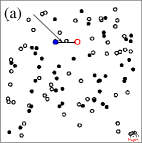
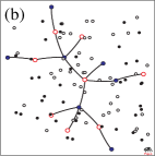
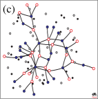
Figure 1: (Color online) Snapshots of the system of mobile agents. Edges between two agents indicate that they already collided with each other: (a) Snapshot after the first collision and (b-c) two subsequent snapshots within one cluster of collisions. Filled nodes (blue) and unfilled nodes (red) represent two different types of nodes, e.g. males and females (see Sec. 6 for details).

We consider periodic boundary conditions and when initialized each agent has a randomly chosen position and moving direction with velocity $v_{0}$. When for the first time two agents collide, the corresponding collision is taken as the first contact in the network, as illustrated in Fig. 1a (see arrow). Letting the agents move and tracking their collisions through time, more and more connections appear (Figs. 1b and 1c). Figure 1 shows the evolution of only one part of the system. Typically, several networks similar to the ones in Figs. 1b and 1c appear during the evolution, each one formed from different single isolated collisions, as the one illustrated in Fig. 1a.

The collision process is based on an event-driven algorithm, i.e. the simulation progresses by means of a time ordered sequence of collision events (diffusion) and between collisions each agent follows a ballistic trajectory[34] (drift). According to the algorithm, collisions take place whenever the distance between the centers of mass of two agents is equal to their diameter.

Since collisions represent social contacts their dynamical rules should fulfill some sociological requirements. Namely, it is known[35] that many social interactions occur more commonly between individuals having already a large number of previous contacts. For instance, in sexual contacts[25] individuals with a larger number of partners are more likely to get new partners. Therefore, we choose a collision rule where the velocity of each agent may increase with the number $k$ of previous contacts, namely

$$\vec{v}(k_{i})=(\bar{v}k_{i}^{\alpha}+v_{0})\vec{\omega},$$ (1)

where $k_{i}$ is the total number of social contacts of agent $i$, $\bar{v}=1\hbox{\ m/s}$ is a constant to assure dimensions of velocity, $\vec{\omega}=(\vec{e}_{x}\cos{\theta}+\vec{e}_{y}\sin{\theta})$ with $\theta$ a random angle and $\vec{e_{x}}$ and $\vec{e_{y}}$ are unit vectors.

The exponent $\alpha$ in Eq. (1) controls the velocity update after each collision. For $\alpha=0$ the velocity of each particle is constant in time, and consequently the kinetic energy density $E=\tfrac{1}{2}\rho v^{2}$ of the system is constant. For $\alpha>0$ the velocity increases with degree $k$. In this range, the value $\alpha=1$ ($|\vec{v}|\propto k$) marks a transition between a sub-linear regime ($\alpha<1$) and a supra-linear regime ($\alpha>1$) with different degree distributions[25]. Throughout the paper we will consider $\alpha=1$ in most of the situations, showing that it produces the suitable dynamics to reproduce real networks of social contacts. It should be noticed that while positive values of $\alpha$ yield dynamical laws which fulfill sociological requirements, the equation of motion (1) is also able to consider completely different situations, where $\alpha<0$, i.e. where the ability to acquire new contacts decreases with the number of previous contacts. In this manuscript, we will focus in the regimes for $\alpha>0$.

As one may notice, contrary to collision interactions where the velocity vector is completely deterministic[36], here momentum is not conserved. This is a consequence not only of the increase of $\vec{v}$ but also of the fact that after one collision the moving direction is randomly selected. The main reason for this random choice is that, as a first approximation it is plausible to assume that social contacts do not determine which social contact will occur next.

Concerning the residence time or ‘age’ parameter $A$, during which the agents remain in the system, if $A\to\infty$, each agent will eventually collide with all the other agents forming a fully connected network. Whereas, when the average residence time of the agents is finite the system will reach a non-trivial quasi-stationary state[37, 38], as described in the next Sec. 3.

The aging scheme considered here is simply parameterized by some threshold in the age of the agents. More precisely, each agent $i$ is initialized with a certain age $A_{i}(0)$ which is a random number uniformly distributed in the interval $[0,T_{\ell}]$ with $T_{\ell}$ being the maximal age an agent may have. Being updated according to $A_{i}(t+\Delta t)=A_{i}(t)+\Delta t$, the age eventually reaches $A_{i}(t)=T_{\ell}$, when the agent $i$ leaves the system, yielding a total residence time $T_{\ell}-A_{i}(0)$. Computationally the replacement of an old agent by a new one is carried out simply by removing all the connections of the old agent and updating its velocity to the initial value $v_{0}$ with a new random direction.

When the average residence time is too small, two agents will have no time to collide at least once, and consequently no network is formed. On the contrary, when $T_{\ell}$ is too large, each agent will cross the entire system and a fully connected network appears. To avoid these two extreme regimes we consider an average residence time which is neither very small nor large when compared with the characteristic time $\tau$ between collisions.

For that, we define a collision rate, as the fraction between the average residence time $T_{\ell}-\langle A(0)\rangle=T_{\ell}/2$, where $\langle x\rangle$ is the average of $x$ over different snapshots in the quasi-stationary state, and the characteristic time $\tau$ of the mean free path defined as

$$\tau=\frac{1}{\sqrt{2\pi}\rho d\langle v\rangle},$$ (2)

where $\langle v\rangle$ is the average velocity of the agents. With this assumptions our collision rate reads

$$\lambda=\frac{T_{\ell}}{2\tau}=\frac{\langle v\rangle T_{\ell}}{2v_{0}\tau_{0}}.$$ (3)

where $\tau_{0}$ is the characteristic time of the system at the beginning when all agents have velocity $v_{0}$.

Before proceeding in characterizing the behavior of such a system it is important to address three last points to understand the parallel between the model and real systems. First, the two-dimensional continuous space where nodes move is not the physical space where individuals travel, meet or establish social acquaintances. Instead, it represents a projection of a highly dimensional Euclidean space whose metric is related to what is called the social distance[12, 39]: the closer two nodes are, the similar their affinities are (same tastes, same behavior, etc.) and therefore more probable to establish an acquaintance, i.e. to collide. It should be stressed that the metric is related to social distance, but also incorporates effects of random factors promoting two persons to meet or establish friendship connections. We have no rigorous explanation for the fact that a two-dimensional projection of such a ‘large’-dimensional space suffices to reproduce empirical data of acquaintances. But the fact is that it does, and therefore for simplicity we will consider a two-dimensional system. One could also consider higher dimensional systems of mobile agents but then the ‘projected’ velocity in Eq.(1) would change.

Second, since the system of mobile agents is used to extract a complex network, the two parameters of the model influence the statistical features of the network structure. Namely, increasing the density $\rho$ confines the accessible region of agents thus promoting the occurrence of collisions among them which are more confined in space. In other words, increasing the density one increases the clustering coefficient[5]. As for $T_{\ell}$, the larger the residence time, the larger the number of collisions an agent may have. Thus, increasing $T_{\ell}$ increases the average number $\langle k\rangle$ of connections.

Finally, in a space of affinities what is the meaning of a velocity? The velocity is in fact a measure of the accessible region of a given agent within this social space which increases, decreases or remains constant after each collision, depending on the value of $\alpha$.

3 The quasi-stationary regime

In this Section we describe in detail the non-trivial topological and dynamical properties of the quasi-stationary (QS) state of the model described in the previous section. As we will see, in the QS state the dynamical and topological quantities fluctuate around an average value after a transient time of the order of $2T_{\ell}$.

Figure 2 illustrates the convergence toward the QS state for two different values of $T_{\ell}$, namely for $T_{\ell}=30.75$ and $T_{\ell}=75.34$. Here, the convergence is characterized by plotting the effective coordination given by the fraction $M/N$ between the total number $M$ of connections and the total number $N$ of nodes (Fig. 2a), the mean energy $\langle E\rangle$ (Fig. 2b) and the mean age $\langle A\rangle$ (Fig. 2c), as function of time $t$. In all three cases, the above quantities increase in the earlier stages of the network growth attaining a maximum value around $t\sim T_{\ell}/2$ where the agents start dying, resulting in the decrease of their values till a minimum at $t=T_{\ell}$. The maximum at $t\sim T_{\ell}/2$ is due to the fact that the agents have on average a life-time equal to $T_{\ell}/2$, while the minimum is due to the extinction of the first ‘generation’ of agents. Notice that, the maximum occurs at $T_{\ell}/2$ due to the choice of the initial uniform distribution of the node age which yields $\langle A(0)\rangle$; in general, for other choice of age distribution one finds a maximum at $t\sim\langle A(0)\rangle$.

Figure 2: Dynamical and topological quantities as function of time $t$: (a) effective coordination $M/N$, (b) mean energy $\langle E\rangle$, (c) average age $\langle A\rangle$. Two different values of the collision rate are plotted: $T_{\ell}=30.75$ and $T_{\ell}=73.34$. In (a) arrows indicate $t=T_{\ell}$, the maximal age an agent may have. In all cases a quasi-stationary state is attained beyond $t\gtrsim 2T_{\ell}$. On the right the PDFs of these quantities are shown (circles), comparing them with Gaussians having the same central moments (solid lines). Here $N=64\times 64$ and $\alpha=1$ (see Eq. (1)).

Figure 3: Correlation $\mu$ between time step $2T_{\ell}$, beyond which the QS is attained, and a subsequent time-step $t\geq 2T_{\ell}$, of the three quantities in Fig. 2: (a) effective coordination $M/N$, (b) mean energy $\langle E\rangle$, (c) average age $\langle T\rangle$. Solid line indicate the result for $T_{\ell}=30.75$, while dashed lines indicate the result for $T_{\ell}=73.34$. Here $N=64\times 64$ and $\alpha=1$.

The average values and corresponding fluctuations of these properties in the QS regime ($t\gtrsim 2T_{\ell}$), depend on $T_{\ell}$, i.e. on $\lambda$ (see Eq. (3)). For large values of $\lambda$ (large $T_{\ell}$) the fluctuation is larger than for small $\lambda$, as can be seen from the probability density functions (PDF) of each quantity shown on the right of Figs. 2a-c. The PDF of the data were computed from the first $2\times 10^{4}$ data points beyond $t\sim 2T_{\ell}$ and are plotted with circles, while a Gaussian with the same average and standard deviation is plotted as a solid line for comparison. While for $T_{\ell}=30.75$ the distributions are approximate Gaussian, for $T_{\ell}=73.34$ there is significant deviation from a Gaussian distribution.

As explained below, between these two values there is a threshold corresponding to a critical collision rate $\lambda_{c}$ separating two different behaviors, one where the system is composed by several small clusters of interconnected nodes and one where all the nodes belong to a single giant cluster. Further, from Fig. 3 one concludes that, beyond $t\gtrsim 2T_{\ell}$, the correlation length is of the order of $T_{\ell}$.

So, although there is no conservation of momentum, the average velocity increasing with time at the beginning, after attaining the QS state $\langle v\rangle$ is almost constant. In the following we assume only values of $\lambda$ in the QS state, taking the average velocity in Eq. (2) as a constant given by the mean of the corresponding PDF distribution. Further, although all quantities, $M/N$, $\langle E\rangle$ and $\langle T\rangle$, characterizing the system in the QS state are functions of $T_{\ell}$, we will choose the adimensional parameter $T_{\ell}/\tau_{0}$ instead, which incorporates also the density of the system.

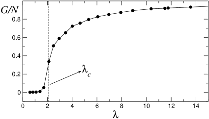
Figure 4: Number $G$ of nodes in the largest cluster of the system of mobile agents as a function of the collision rate $\lambda$. At $\lambda_{c}\simeq 2.04$ one sees the emergence of a giant cluster with $G/N\sim 1$ (see Sec. 5). Here $N=128\times 128$ and $\alpha=1$.

As said above, by varying the collision rate $\lambda$, one finds a critical value $\lambda_{c}$ marking a transition from a state composed by several small clusters to a state where a giant cluster emerges after attaining the QS state. In Fig. 4 we plot the fraction $G/N$ between the number $G$ of nodes in the largest cluster and the total number $N$ of nodes. Clearly, beyond $\lambda_{c}\simeq 2.04$ one sees the emergence of a giant cluster. In the next Section 4 we describe and discuss the topological properties for this largest cluster and in Section 5 we characterize the percolation transition occurring at $\lambda_{c}$.

4 Properties of the network

In this section we will study the degree distribution $P(k)$, the clustering distributions $C(k)$ characterizing the cliquishness of the agents neighborhoods, and the average path length $\ell$ in the QS state.

The average degree $\langle k\rangle$ per agent is a function of both the collision rate $\lambda$ and rescaled maximal age $T_{\ell}/\tau_{0}$ as shown for two different values of $\rho$ in Fig. 5a and 5b respectively. From Fig. 5a one sees that $\langle k\rangle=\lambda/2$ independently on the density $\rho$, while as a function of $T_{\ell}/\tau_{0}$ the average degree increases exponentially with an exponent depending on the density. These two plots are important not only to study the topological features of the agent model, but also to find the appropriate values when modeling real networks as will be explained in Section 6.

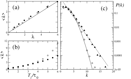
Figure 5: Average degree $\langle k\rangle$ as a function of (a) the collision rate $\lambda$ and of (b) the maximal age $T_{\ell}/\tau_{0}$ for two values of the density, $\rho=0.02$ (white circles) and $\rho=0.2$ (black circles), both with $\alpha=1$. The solid line in (a) indicates $\lambda=2\langle k\rangle$. (c) Degree distribution of the giant cluster in the QS state for two different velocity updates (see Eq. (1)): $\alpha=0$ (triangles) with $T_{\ell}/\tau_{0}=9.5$, where the velocity modulus is always constant and $\alpha=1$ (diamonds) with $T_{\ell}/\tau_{0}=3$, where velocity modulus increases linearly with the number of previous connections. Measuring in each case $\langle k\rangle$ in the system and introducing its value in Eqs. (4) and (5), yields the suitable fits for each $\alpha$ value, namely a Poisson distribution (solid line) with $\langle k\rangle=2.52$ and an exponential distribution (dashed line) with $\langle k\rangle=2.62$. In all cases, averages over $100$ iterations were taken after attaining the QS state for a system of $N=10^{4}$ agents.

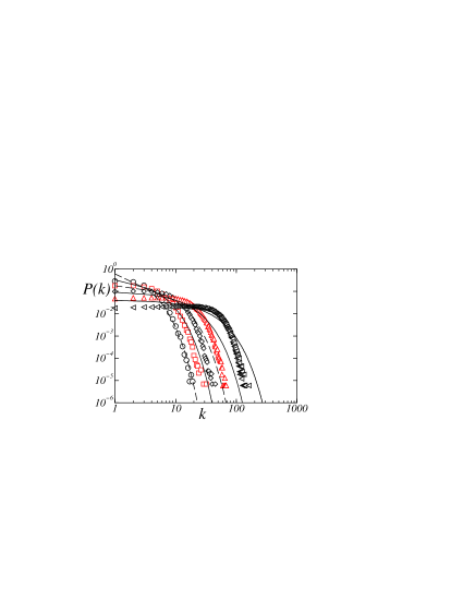
Figure 6: (a) Degree distribution of the giant cluster in the $QS$ state, for several values of $\lambda=5.24,8.04,13.04,23.76$ and $57.36$ (symbols). Lines indicate the corresponding exponential fit with Eq. (5). Here $N=64\times 64$ and $\alpha=1$. For other system sizes the results are similar.

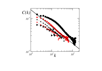
Figure 7: Clustering coefficient distribution for the same simulations of Fig. 6, namely for (left to right) $\lambda=5.24,8.04,13.04,23.76$ and $57.36$. The solid line is a guide to the eye with slope $1/2$ (see details in text). Here $\alpha=1$, $N=128\times 128$ and averages over $100$ realizations were taken.

In Fig. 5c we compute the degree distribution $P(k)$, by counting the fraction of nodes having $k$ neighbors. Two different velocity updates are illustrated here, namely $\alpha=0$ (triangles) and $\alpha=1$ (diamonds). Clearly, the degree distribution depends strongly on the collision update rule, i.e. on the value of $\alpha$ in Eq. (1).

More precisely, for $\alpha=0$, the velocity of each agent is always constant, the resulting degree distribution being a consequence of the effective time[24] $t_{\hbox{eff}}=3T_{\ell}/8$ to create links and of the collision rate, yielding a Poisson distribution

$$P(k)=\frac{\langle k\rangle^{k}}{k!}e^{-\langle k\rangle}.$$ (4)

For this value $\alpha=0$, the degree distribution was calculated for a fixed value of $T_{l}/\tau_{0}=9.5$ the resulting network has $\langle k\rangle=2.52$, introducing this value in eq.4, we obtain the solid line in Fig. 5c, which shows that the degree distribution of the network is well aproximated by a poissonian. In this way, one can argue that for $\alpha=0$ the system produces a two-dimensional geometric random graph [40] in the QS state.

For $\alpha=1$ the velocity in Eq. (1) increases linearly with the number of previous collisions. As we will see, this kind of dynamics reveals to be most suited to reproduce the statistical features of real social networks (see Sec. 6). In this case, the effective residence time is uniformly distributed (see Sec. 2), yielding an exponential velocity distribution and consequently an exponential degree distribution

$$P(k)=\frac{1}{\langle k\rangle-1}e^{-(\frac{k-1}{\langle k\rangle-1})}.$$ (5)

In Fig. 5 the dashed line indicates the distribution in Eq. (5) with $\langle k\rangle=2.62$, which results from a value of $T_{l}/\tau_{0}=3.0$ used in the numerical simulation (triangles). So, for this value $\alpha=1$ the agent model is capable of producing a two-dimensional exponential graph in the QS state.

In the following we will consider the value $\alpha=1$ in Eq. (1) and study how the degree distribution depends on the collision rate $\lambda$. Figure 6 shows the degree distribution in the QS state for $\lambda=5.24$ (circles), $8.04$ (squares), $13.04$ (diamonds), $23.76$ (up triangles) and $57.36$ (left triangles), plotting with lines the exponential in Eq. (5) evaluated with the corresponding $\langle k\rangle$. As one sees, while for small $\lambda$ the exponential expression fits well the observed degree distributions, for larger $\langle k\rangle$ the numerical results have a lower cutoff than the analytical expression. Therefore, one concludes that the agent model is able to reproduce exponential distributions for low values of the collision rate ($\lambda<10$), and that other non-trivial distributions appear increasing the collision rate. The latest ones are the ones observed in empirical social networks (see Sec. 6).

Another property of interest to characterize the network is its clustering coefficient. The local clustering coefficient $C_{i}$ of a vertex $i$ with degree $k_{i}$ measures its cliquishness and is defined as the quotient between the number $w_{i}$ of triangles (cycles composed by three edges) and the total number of triangles,

$$C_{i}=\frac{2w_{i}}{k_{i}(k_{i}-1)}.$$ (6)

To uncover hierarchical properties of the network, one usually[41] computes the clustering coefficient as a function of the degree $k$, namely

$$C(k)=\frac{2\langle w(k)\rangle}{k(k-1)},$$ (7)

where $\langle w(k)\rangle$ is the average number of triangles of a node with degree $k$.

Figure 7 shows the mean degree-dependent clustering coefficient $C(k)$ for the same mobile agents systems of Fig. 6. It is interesting to note that, in contrast to random graphs, which have a clustering coefficient independent of $k$, here we observe a dependence of the form $\sim k^{-\alpha}$ with $\alpha\in[0.4,0.6]$. In other words, Fig. (8) shows that the clustering coefficient decreases with the degree, a feature which indicates the existence of an underlying hierarchical structure[42].

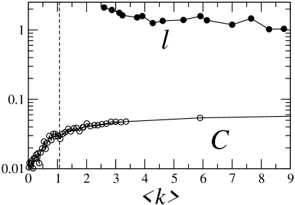
Figure 8: Average path length $\ell$ ($\bullet$) and clustering coefficients $C$ ($\circ$) as functions of the average degree. Here $\rho=0.02$.

To end this Section, we study two other topological quantities, namely the average shortest path length $\ell$ and the average clustering coefficient $C$. As one knows [5], knowing the values of these topological quantities one is able to ascertain for small-world effects.

The average clustering coefficient is defined as the average of the local clustering coefficients $C_{i}$ in Eq. (6) for all $i=1,\dots,N$, and the average shortest distance $\ell$ is given by the average minimal number of edges joining two randomly chosen nodes.

To investigate small-world effects in our system, we compare the networks of the model of mobile agents with random networks having the same number $N$ of nodes and where each pair of nodes is connected with a probability $p=2M/(N(N-1))$. With this probability one obtains a random network with approximately the same effective coordination $M/N$ (same $\langle k\rangle$) as the one observed in the model of mobile agents.

Figure 8 shows these two quantities as a function of the average degree $\langle k\rangle$. The clustering coefficient increases with $\langle k\rangle$, and beyond the emergence of the giant component ($\langle k\rangle>\lambda_{c}/2=k_{c}$) it slowly converges to a value $C_{\infty}\lesssim 0.1$. The vertical line shows the critical point $k_{c}=1.02$. As for the average path length $\ell$ one observes a slow decrease with the average degree. Notice that for very low values of $\langle k\rangle$ (not shown) there are no sufficient edges to guarantee a meaningful average path length, in particular, below the transition at $k_{c}$ the system is divided in several different clusters, which leads to an undefined $\ell$.

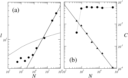
Figure 9: Size dependence of the networks of mobile agents. (a) Shortest path length $\ell$ as a function of the system size $N$, for $T_{l}/\tau_{0}=5.02$, compared to $\ln{N}$ (dashed lines). For large network sizes the solid line indicates a fit $\ell=e^{-3}\sqrt{N}$ (see text). (b) Average clustering coefficient ($C$) as a function of $N$ for the agent model (bullets) compared to the corresponding random graph with the same $\langle k\rangle$ (triangles), having a fit (solid line) of $C\sim 1/N$. Here $\rho=0.02$.

In Fig. 9a, the average path length is small compared to the system size. Moreover, as seen in Fig. 9b the cluster coefficient in the agent model (circles) is much larger than in the random counterparts (triangles). However, the networks generated by the model of mobile agents are not small-world, since to have the small-world property[3] it is also required that the increase of the shortest path length with the system size is not faster than $\ln{N}$. From Fig. 9a one sees that this is only true for small system sizes ($N<10^{4}$). For larger systems, the fitted numerical results yield $\ell=e^{-3}\sqrt{N}$.

In Fig. 9b one sees the behavior of the average cluster coefficient when the system size is increased. Interestingly, one clearly sees an independence on $N$, beyond $N>10^{3}$, where $C\sim 0.08$. For higher density values $\rho$ this $N$-independent value of $C$ increases. This result is quite in contrast to random graphs which scales with $1/N$, as illustrated in Fig. 9b with triangles.

Having characterized the features of the system beyond the transition at $\lambda_{c}$, where a giant cluster emerges, in the next Section we focus on the properties of this transition.

5 Critical behavior

The emergence of the giant cluster for an exponential network has been studied by Molloy and Reed [43] or equivalently using the generating function formalism by Newman  [44]. In both cases the transition belongs to the universality class of mean field percolation, in contrast to the agents model which is in the universality class of two-dimensional percolation, as we will show in this Section.

The percolation transition is the abrupt change, at a particular critical value $\lambda_{c}$, from a state composed by several small clusters to a state where a giant cluster dominates. A cluster is defined as a group of connected agents. Isolated agents are regarded as clusters of size unity and any cluster consisting of $s$ connected agents is called an $s$-cluster. We borrow the notation from Stauffer’s book on percolation theory [45] and define here $n_{s}=N_{s}/N$ as the number of $s$-clusters per agent, where $N_{s}$ is the number of clusters of size $s$ and $N$ the total number of agents in the system.

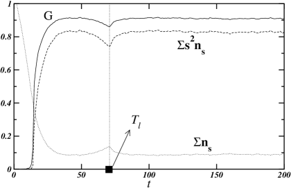
Figure 10: Cluster quantities as function of time $t$: Number $G$ of agents belonging to the largest cluster (solid line), total number of clusters $\Sigma_{s}n_{s}$ (dotted line) and size-averaged mean cluster size $\Sigma_{s}s^{2}n_{s}$ (dashed line). All quantities are normalized by $N$. Here $N=128\times 128$ and $\lambda=13.04$.

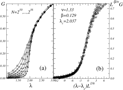
Figure 11: (a) Fractions of sites in the largest cluster $G/N$ as function of $\lambda$. The numerical results where extracted in the $QS$ state for a fixed value of $T_{l}/\tau_{0}$, with $N=32^{2},46^{2},92^{2},128^{2}$ and $256^{2}$. (b) Confirmation of the scaling relation in Eq. (8), for the system sizes $N=2^{10},2^{11},\dots,2^{16}$ and the values of $\beta$ and $\nu$ reported in Tab. 1 at the critical value $\lambda_{c}=2.04$.

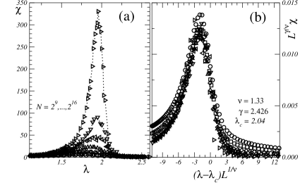
Figure 12: (a) Size-averaged mean cluster size $\sum s^{2}n_{s}$ as a function of $\lambda$ for the same system sizes as in Fig. 11a. (b) Confirmation of the scaling relation of Eq. (9), for the same system sizes the values of $\gamma$ and $\nu$ reported in Tab. 1 and $\lambda_{c}=2.04$.

In Fig. 10 we show the time evolution of the size $G$ of the largest cluster (see also Fig. 4), together with the total number $\sum n_{s}$ of clusters and the corresponding size-averaged mean cluster size $\sum s^{2}n_{s}$. At the beginning the size of the giant cluster and the size of the mean cluster increase till $t=T_{\ell}/2$, corresponding to a complementary decrease of the number of clusters. Beyond this instant, agents which have an average residence time of $T_{\ell}/2$, start to leave the system losing all their connections, and therefore both the size of the giant cluster and the mean cluster size start to decrease till $t=T_{\ell}$. Thereafter, all the first generation of nodes has left the system, and the evolution converges rapidly to the QS state where all quantities present constant values, apart small fluctuations. For other values of $T_{\ell}$, i.e. of the collision rate $\lambda$, one observes the same behavior of the above quantities, reaching the QS state at different values.

The next step is to calculate for a given value of $T_{l}$, the value of $\lambda$ in the $QS$ state and average at different times the value of $G$. The result is plotted in Fig. 11a for different system sizes. Simultaneously, the value of $\chi$, given by the size-averaged mean cluster size without the largest cluster, is also calculated. The result is shown in Fig. 12a.

In general, according to the standard scaling theory [46], we expect $G$ (Fig. 11a) and $\chi$ (Fig. 12a) to follow

$$G=L^{-\beta/\nu}F[(\lambda-\lambda_{c})L^{-1/\nu}]$$ (8)

$$\chi=L^{\gamma/\nu}G[(\lambda-\lambda_{c})L^{-1/\nu}].$$ (9)

where $L$ is the linear size of the system ($N=L^{2}$). This is confirmed by the collapses of the curves near the the critical point, i.e. $\lambda-\lambda_{c}\sim 0$, as illustrated in Figs. 11b and  12b respectively, for the values of $\nu$, $\beta$, and $\gamma$ reported in the central column of Tab. 1, with $\lambda_{c}=2.04$.

	$MF$	mobile agents	Percolation (2D)[45]
$\nu$	$0.5$	$1.3\pm 0.1$	$4/3\sim 1.33$
$\gamma$	$1$	$2.4\pm 0.1$	$43/18\sim 2.39$
$\beta$	$1$	$0.13\pm 0.01$	$5/36\sim 0.139$
$\sigma$	$0.5$	$0.40\pm 0.01$	$36/91\sim 0.397$

Table 1: Critical exponents related to the emergence of the giant cluster in a random graph model (percolation $MF$), for the network of mobile agents presented here, compared to the exact results of percolation $2D$.

In order to test the scaling relation obtained above, we compute the number $n_{s}(\lambda)$ of clusters of size $s$ as a function of $\lambda$, as shown in the inset of Fig. 13, for $N=2^{16}$ agents. For the computation, we calculate bins (power-two) of the cluster size distribution at different values of $\lambda$, ignoring the first four bins, that is the sizes, $1$, $2-3$, $4-7$, and $8-15$, since for such small clusters scaling is not good[45]. We take the next $4$ bins, i.e. $s$-values in the ranges $[16-31]$, $[32-63]$, $[64-127]$ and $[128-255]$ and plot them for different $\lambda$.

The main plot in Fig. 13 shows the result after scaling. Here, for each bin we take the ratio $n_{s}(\lambda)/n_{s}(\lambda_{c})$ as a function of $(\lambda-\lambda_{c})s^{\sigma}$ using $s$ as the geometric average over the two extremes of the bin ranges enumerated above. Performing this scaling we obtain

$$\sigma=\frac{1}{\beta+\gamma},$$ (10)

using the values of $\beta$, $\gamma$ and $\lambda_{c}$ obtained previously (see Tab. 1).

Equation (10), confirms that the scaling relation of the phase transition belongs to the universality class of percolation. It is known that the emergence of a giant cluster for a random graph depends on $\langle k\rangle$ with its critical value at $\langle k\rangle_{c}=1$, and the phase transition belongs in the same universality class as mean field percolation [47], whose exponents are given in the first column of Tab. 1. However, for the agent model one observes the same emergence of the giant cluster at $\langle k\rangle_{c}=0.5\lambda_{c}=1.02$ and the universality class corresponds to $2d$-percolation, as shown in Tab. 1.

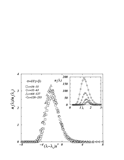
Figure 13: Collapse of the curves from the inset, plotting $n_{s}/n_{s}(\lambda_{c})$ as a function of $(\lambda-\lambda_{c})s^{\sigma}$ (see text). In both cases curves were plotted for cluster sizes in the ranges $[16,31]$, $[32-63]$, $[64-127]$, and $[128-255]$.

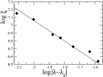
Figure 14: Correlation length $\xi$ as function of $\lambda-\lambda_{c}$. Symbols indicate the result of simulations performed for different values of $\lambda$ and the solid line has a slope of $\nu=-1.3$.

Before ending this Section, we stress that the correlation exponent $\nu$ presented in Tab. 1 is obtained from finite size scaling. This exponent can be also explicitly calculated from the linear size of clusters (see [45]), namely by computing the correlation length $\xi(\lambda)\sim|\lambda-\lambda_{c}|^{-\nu}$. The result is shown in Fig. 14, where the solid line has a slope of $-1.3$ yielding a correlation exponent in agreement with the previous results (see Tab. 1). Since the agents move on a two-dimensional plane and have only a finite life time, they can only establish connections within a restricted vicinity, and this effect corresponds to a connectivity which is short range. Thus, although the clusters in the agent model are not quenched in time, the underlying dynamics yields a short range $2d$-percolation.

6 Real network of social interactions

In the previous Section we described the main characteristics of the model of mobile agents in the QS regime, namely an exponential degree distribution and a transition to percolation for a certain critical collision rate, beyond which no small-world effects are observed. In this Section we analyze a real social network and show that its topological features are well reproduced by our model. In particular, we show that the statistical features observed for the empirical networks are well reproduced with parameter values beyond the transition to percolation.

The empirical data comprehend an extensive study done within the National Longitudinal Study of Adolescent Health (AddHealth) [48] at the Carolina Population Center, concerning $84$ American schools. The aim is to allow social network researchers interested in general structural properties of friendship networks to study the structural and topological properties of social networks [32]. All data are constructed from the in-school questionnaire from a total of $90118$ students which responded to it in a survey between 1994 and 1995. The students are separated by the school they belong to in a total of $84$ schools whose corresponding network sizes range from $\sim 100$ to $\sim 2000$ students.

Figure 15 shows several plots of the degree distributions in nine of the schools (circles) compared to the distributions obtained with the agent model (solid lines) for the same number of agents. The values for the collision rate in the simulations were taken from $\lambda=2\langle k\rangle$ where the average degree is the one found in the corresponding school. As one sees, in all cases the tails of the distributions are well fitted by the model.

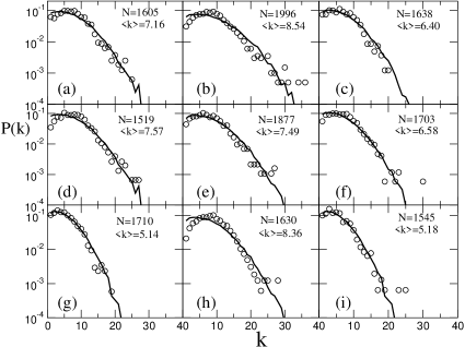
Figure 15: Reproducing the distribution of friendship acquaintances in empirical social networks [48] with the agent model. In all cases circles represent the empirical data, while solid lines indicate the result of the model of mobile agents.

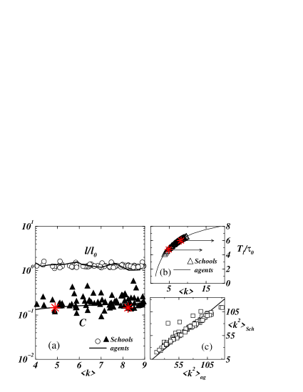
Figure 16: (Color online) (a) Average shortest path length $l$ and clustering coefficient $C$ as functions of the average degree $\langle k\rangle$. Empirical data (symbols) compared to simulations (solid lines). (b) Plot of $T_{l}/\tau_{o}$ as a function of $\langle k\rangle$ for the agents models (solid line). Stars illustrate two particular schools for Figs. 15 having $T_{l}/\tau_{o}=4.75$ (school 1) and $6.0$ (school 2) respectively. (c) Second moment $\langle k^{2}\rangle$ for each school vs. the second moment of the corresponding simulation with the agent model (solid line has slope one). In all cases $\rho=0.1$.

Clearly, the agent model reproduces the degree distribution observed in schools, by introducing the same average degree found in real data. The agent model is not only able to reproduce these degree distributions, shown in Fig. 15, but also the corresponding clustering coefficient and the shortest path length.

Figure 16a shows for each schools (symbols) the average shortest path length $\ell$ (circles), and the clustering coefficient (triangles). Solid lines indicate the results obtained for the agent model using the same values of $\langle k\rangle$, averaged over $100$ realizations with $N=2209$ and $\rho=0.1$. Since $\ell$ depends on the network size, it is divided by the shortest path length $l_{0}$ of a random graph with the same average degree and size. Clearly, the agent model predicts accurately both the clustering coefficient and the shortest path length for the same average degree.

By computing the average degree $\langle k\rangle$ of each school one is able to obtain the value of $T_{l}/\tau_{0}$ for which the agent model reproduces properly the empirical data, as illustrated in Fig. 16b. Here solid lines indicate the calculated curve from the agent model, while triangles indicate the values of $T_{l}/\tau_{0}$ chosen to reproduce the social network of the schools with the resulting value of $\langle k\rangle$. Moreover, the second moment $\langle k^{2}\rangle_{ag}$ obtained with the simulations of the agent model is rescaled by the same quantity $\langle k^{2}\rangle_{Sch}$ measured for the empirical school networks, as shown in Fig. 16c.

In other words, a strong point of our model is that since the average degree varies monotonically with $\lambda$ one can associate a particular value of the collision rate to each school. The collision rate and in particular this parameterization for the collision rate depends weakly on the network size. Here we neglect this dependence, as a first approximation. Using this one-to-one correspondence one is able to compare the topological quantities between the schools and the model of mobile agents.

Notice that, the Add Health in-school friendship nomination data was constructed from a questionnaire where each student listed their in-school friends by order of importance (best friend first) and to each of the friends they indicate which kinds of contacts they had in the last seven days, out from five possible choices. According to the number of different kinds of acquaintances a weight from $1$ to $5$ is attributed to each social contact. Moreover, since the questionnaires are based on the information given by one agent, the networks are directed. Here, we each social contact. Moreover we assume as a first approximation that social contacts are unweighted. Using all the information concerning these empirical networks [32] a more detailed study of the structure of these networks will be presented elsewhere[49].

Figure 17: Cumulative degree distribution of the number $k$ of sexual partners in a real empirical network of sexual contacts (triangles) with $250$ individuals, compared to the simulation of the agent model (solid line), the dotted line is a guide to the eye with slope $2$. Here $N=4096$, $T_{l}/\tau_{o}=5.5$ and $\langle k\rangle=7.32$ and the average size of the resulting sexual network is $220$.

Finally, we stress that with a slight extension of the model it is possible to reproduce subsets of social connections, e.g. sexual contacts, having particular features different from the entire network of all the acquaintances. For instance, in the case of sexual contacts the degree distribution is commonly a power-law [21]. Figure 17 shows the degree distribution of a sexual contact network (triangles) extracted from a tracing study for HIV tests in Colorado Springs[50]. The dashed line indicates the result obtained for a network of all social contacts simulated with the agent model, while the solid line is the degree distribution of a subset of contacts from the social network.

The contacts in the subset are chosen by assigning to each agent an intrinsic property, say a fitness, which enables one to select from all the social contacts the ones of particular interest, in this case sexual contacts. The fitness is defined by a given number and, when two agents form a link, this link is marked as a ’sexual contact’ if the sum of agents fitnesses, $\xi_{i}+\xi_{j}$, is greater than a given threshold. The initial distribution of the fitness is assigned to the agents following an exponential distribution and the threshold is $\ln{N}/2$, following the scheme of intrinsic fitness proposed in another context by Caldarelli et. al. [51]. Interestingly, one is able to extract from the typical distributions of social contacts shown in this Section, which are not scale-free, power-law distributions in QS state which resemble much the ones observed in real networks of sexual contacts (see also Ref. [25]).

7 Conclusions

In this paper we introduce an approach to construct networks of complex interactions from a model of mobile agents. The network is constructed by keeping track of the collision between the mobile agents. Introducing an aging scheme the network attains a QS regime, characterized by almost constant topological and dynamical quantities which fluctuate slightly around an average value. Typically, the networks constructed with the agent model, while having small path lengths and large clustering coefficients, do not show small-world effects, since the average path length does not scale logarithmically with $N$.

The control parameters of the model are the density of the agents and the maximal residence time the agents may have. With these two parameters it is possible to define a collision rate which, for a critical value, marks a percolation transition whose exponents are the ones of two-dimensional percolation. While for small collision rates, the degree distributions are approximately exponential, for larger values of the collision rate they strongly deviate from the exponential approximation yielding a non-trivial degree distribution. Surprisingly, these degree distributions are precisely the same as the ones observed in real social networks of empirical data. This empirical data has many other informations which were not used in this study, namely the gender of the agent and the ‘direction’ and ‘weight’ of the acquaintance. Therefore future investigations on the context of network analysis of this recent empirical data could be interesting for sociological purposes[49].

Moreover, we have shown that the agent model is also able to reproduce networks having only social contacts of particular nature, e.g. sexual contacts. In the particular case of sexual contacts it was found [21] that the distribution of sexual partners has a power-law tail. The dynamical reasons underlying this discrepancy between the ‘total’ number of social contacts, with exponential distributions, and the particular number of sexual contacts, with power-law tails, is not yet explained.

References

- [1] M.E.J. Newman, SIAM Rev. 45, 167 (2003).
- [2] S.N. Dorogovtsev and J.F.F. Mendes, Adv. Phys. 51, 1079 (2002).
- [3] R. Albert and A.-L. Barabási, Rev. Mod. Phys. 74, 47 (2002).
- [4] B. Bollobás, Modern Graph Theory (Springer, New York, 1998).
- [5] D.J. Watts and S.H. Strogatz, Nature 393, 440 (1998).
- [6] P.G. Lind, M.C. González and H.J. Herrmann, Phys. Rev. E 72, 056127 (2005); cond-mat/0504241.
- [7] P.L. Krapivsky and S. Redner, Phys. Rev. Lett. 90, 238701 (2003).
- [8] A. Rogers, Phys. Rev. Lett. 90, 158103 (2003).
- [9] R. Pastor-Satorras and A. Vespignani, Phys. Rev. E 65, 036104 (2002).
- [10] D.Y.C. Chan, B.D. Hughes, A.S. Leong and W.J. Reed, Phys. Rev. E 68, 066124 (2003).
- [11] J. Davidsen, H. Ebel, and S. Bornholdt, Phys. Rev. Lett. 88, 128701 (2002).
- [12] M. Boguñá, R. Pastor-Satorras, Albert Díaz-Guilera, and Alex Arenas Phys. Rev. E. 70, 056122 (2004).
- [13] M.E.J. Newman Phys. Rev. Lett. 89, 208701 (2002).
- [14] R. Pastor-Satorras and A. Vespignani, Evolution and Structure of the Internet: A Statistical Physics Approach, (Princ. Univ. Press, Princeton, 1999).
- [15] M.E.J. Newman, Proc. Natl. Acad. Sci. 98, 404 (2001).
- [16] H. Jeong, B. Tombor, R. Albert and A.-L. Barabási, Nature 407, 651 (2000).
- [17] H. Jeong, S.P. Mason, A.-L. Barabási and Z.N. Oltvai, Nature 411, 41 (2001).
- [18] D.J. Watts, Small Worlds: The Dynamics of Networks Between Order and Randomness, (Camb. Univ. Press, Cambridge, 2004).
- [19] Airport Council International, ACI Annual Worldwide Airports Traffic Reports (Airport Counc. Int., Geneva, 1999).
- [20] “Virtual Round Table on ten leading questions for network research”, Eur. Phys. J. B 38, 143 (2004).
- [21] F. Liljeros, C.R. Edling, L.A.N. Amaral and H.E. Stanley, Nature 411, 907 (2001).
- [22] A. Schneeberger, C. Mercer, S.A.J. Gregson, N.M. Ferguson, C.A. Nyamukapa, R.M. Anderson, A.M. Johnson, G.P. Garnett, Sex. Trans. Dis. 31, 380 (2004).
- [23] E. Eisenberg and E.Y. Levanon, Phys. Rev. Lett. 91, 138701 (2003).
- [24] M.C. González, P.G. Lind and H.J. Herrmann Phys. Rev. Lett. 96, 088702 (2006); cond-mat/0602091.
- [25] M.C. González, P.G. Lind and H.J. Herrmann, Eur. Phys. J. B 49, 371-376 (2006); physics/0508145.
- [26] S.H. Strogatz, Nature 410, 268 (2001).
- [27] K.T.D. Eames and M.J. Keeling, Proc. Nat. Ac. Sci. 99, 13330 (2002).
- [28] L.C. Freeman, The Development of Social Network Analysis (Vancouver, Canada, 2004).
- [29] M.C. González and H.J. Herrmann, Physica A 340 741 (2004); cond-mat/0402443.
- [30] M.C. González, H.J. Herrmann and A.D. Araújo, Physica A 356, 100 (2005); cond-mat/0502665.
- [31] E.M. Jin, M. Girvan, M.E.J. Newman, Phys. Rev. E 64, 046132 (2001).
- [32] P.S. Bearman, J. Moody and K. Stovel, Am.J. of Soc. 110, 44 (2004).
- [33] T. Pöschel and S. Luding, Granular Gases, (Lecture Notes in Physics, 564, Springer-Verlag, 2001)
- [34] D.C. Rapaport, The Art of molecular dynamics simulation, (Cambridge University Press, Cambridge, 1995).
- [35] E.O. Laumann, J.H.Gagnon, R.T Michaels, Organization of Sexuality, (University of Chicago Press, 1994).
- [36] D. ben-Avraham, E. Ben-Naim, K. Lindenberg, A. Rosas, Phys. Rev. E 68, 050103 (2003).
- [37] L.A.N. Amaral, A. Scala, M. Barthélémy, H.E. Stanley, Proc. Natl. Acad. Sci. 21, 11149 (2000).
- [38] S.N. Dorogovtsev, J.F.F. Mendes, Phys. Rev. E 62, 1842-1845 (2000).
- [39] D.J. Watts, P.S. Dodds, M.E.J. Newman, Science 196, 1302-1305 (2002).
- [40] J. Dall, M. Christensen, Phys. Rev. E 66, 016121 (2002).
- [41] E. Ravasz, A.-L. Barabási, Phys. Rev. E 67, 026112 (2003).
- [42] G. Caldarelli, R. Pastor-Satorras and A. Vespignani, Eur. Phys. J. B 38, 183-186 (2004).
- [43] M. Molloy and B. Reed, Comb. Probab. Comput. 7, 295 (1998).
- [44] D.S. Callaway, J.E. Hopcroft, J.M. Kleinberg, M.E.J. Newman and S.H. Strogatz, Phys. Rev. E 64, 042902 (2001).
- [45] D. Stauffer, Introduction to Percolation Theory, (Taylor & Francis, London, 1985).
- [46] M.E.J.Newman and G. T. Barkema Monte Carlo methods in statistical physics, (Clarendon Press, Oxford, 1999).
- [47] K. Christensen, R. Donangelo, B. Koiler, and K. Sneppen, Phys. Rev. Lett. 81, 2380 (1998).
- [48] This research uses data from Add Health, a program project designed by J. Richard Udry, Peter S. Bearman, and Kathleen Mullan Harris, and funded by a grant from the National Institute of Child Health and Human Developtment (P01-HD31921).
- [49] M.C. González, H.J. Herrmann, J. Kertész, T. Vicsek, in preparation (2006).
- [50] J.J. Potterat, L. Phillips-Plummer, S.Q. Muth, R.B. Rothenberg, D.E. Woodhouse, T.S. Maldonado-Long, H.P. Zimmerman, J.B. Muth, Sex. Transm. Infect. 78, i159 (2002).
- [51] G. Caldarelli, A. Capocci, P. De Los Rios, M.A. Muñoz, Phys. Rev. Lett. 89, 258702 (2002).