A new view on relativity:
Part 2. Relativistic dynamics

The Lorentz transformations are represented on the ball of relativistically admissible velocities by Einstein velocity addition and rotations. This representation is by projective maps. The relativistic dynamic equation can be derived by introducing a new principle which is analogous to the Einstein’s Equivalence Principle, but can be applied for any force. By this principle, the relativistic dynamic equation is defined by an element of the Lie algebra of the above representation.

If we introduce a new dynamic variable, called symmetric velocity, the above representation becomes a representation by conformal, instead of projective maps. In this variable, the relativistic dynamic equation for systems with an invariant plane, becomes a non-linear analytic equation in one complex variable. We obtain explicit solutions for the motion of a charge in uniform, mutually perpendicular electric and magnetic fields.

By the above principle, we show that the relativistic dynamic equation for the four-velocity leads to an analog of the electromagnetic tensor. This indicates that force in special relativity is described by a differential two-form.

PACS: 03.30.+p ; 03.50-z.

1 Introduction

In Part 1 we have shown that from the Principle of Relativity alone, we can infer that there are only two possibilities for space time transformations between inertial systems: the Galilean transformations or the Lorentz transformations. In Special Relativity we use the Lorentz transformation and obtain interval conservation. We also show that the set of all relativistically allowed velocities is a ball $D_{v}\in R^{3}$ of radius $c$-the speed of light. We have shown that similar results hold for proper-velocity-time transformations between accelerated systems.

If an object moves in an inertial system $K^{\prime}$ with uniform velocity $\mathbf{u}$ and $K^{\prime}$ moves parallel to $K$ with relative velocity $\mathbf{b}$, then in system $K$ the object has uniform velocity $\mathbf{b}\oplus\mathbf{u}$, the relativistic sum of $\mathbf{b}$ and $\mathbf{u},$ defined as

$$\mathbf{b}\oplus\mathbf{u}=\frac{\mathbf{b}+\mathbf{u}_{\|}+\alpha\mathbf{u}_{\bot}}{1+\frac{\langle\mathbf{b}|\mathbf{u}\rangle}{c^{2}}},$$ (1)

where $\mathbf{u}_{\|}$ denotes the component of $\mathbf{u}$ parallel to $\mathbf{b}$, $\mathbf{u}_{\bot}$ denotes the component of $\mathbf{u}$ perpendicular to $\mathbf{b}$ and $\alpha=\sqrt{1-|\mathbf{b}|^{2}/c^{2}}$. This is the well-known Einstein velocity addition formula. Note that the velocity addition is commutative only for parallel velocities. The Lorentz transformation preserves the velocity ball $D_{v}$ and acts on it by

$$\varphi_{\mathbf{b}}(\mathbf{u})=\mathbf{b}\oplus\mathbf{u}.$$ (2)

It can be shown [2] that the map $\varphi_{\mathbf{b}}$ is a projective (preserving line segments) automorphism of $D_{v}$.

We denote by $Aut_{p}(D_{v})$ the group of all projective automorphisms of the domain $D_{v}$. The map $\varphi_{\mathbf{b}}$ belongs to $Aut_{p}(D_{v})$. Let $\psi$ be any projective automorphism of $D_{v}$. Set $\mathbf{b}=\psi(0)$ and $U=\varphi_{\mathbf{b}}^{-1}\psi$. Then $U$ is an isometry and represented by an orthogonal matrix. Thus, the group $Aut_{p}(D_{v})$ of all projective automorphisms has the characterization

$$Aut_{p}(D_{v})=\{\varphi_{\mathbf{b}}U:\mathbf{b}\in D_{v},\;U\in O(3)\}.$$ (3)

This group represents the velocity transformation between two arbitrary inertial systems and provides a representation of the Lorentz group.

Now we are going to adapt Newton’s classical dynamics law

$$\mathbf{F}=m\mathbf{a}=m\frac{d\mathbf{v}}{dt}$$

to special relativity. By definition, a force generates a change of velocity. Since in special relativity the velocity must remain in $D_{v}$, the changes caused by the force cannot take the velocity out of $D_{v}$. This implies that on the boundary of the domain $D_{v}$, the changes caused by the force cannot have a non-zero component normal to the boundary of the domain and facing outward. One of the common ways to solve this problem is to assume that the mass $m$ approaches infinity as the velocity approaches the boundary of $D_{v}$.

We consider the mass of an object to be an intrinsic characteristic of the object. We therefore keep the mass constant and equal to the so-called rest-mass $m_{0}$. Under such an assumption we must give up the property that the force on an object is independent of the velocity of the object, since such a force would take the velocity out of $D_{v}$. Note that also in non-relativistic mechanics we have forces which depend on the velocity, like friction and the magnetic force.

To derive the relativistic dynamics equation, we must introduce a new axiom which will allow us to derive such an equation. For alternative axioms used by others, see Rindler [5], p.109. Based on this new axiom, we will derive a relativistic dynamics equation. Our equation agrees with the known relativistic dynamics equation obtained by different assumptions. The difference will be only in the interpretation and the derivation of the equation.

2 Extended Partial Equivalence Principle —$EP^{2}$

We base our additional axiom for relativistic dynamics on Einstein’s Equivalence Principle. In the context of flat space-time, the Principle of Equivalence states that “the laws of physics have the same form in a uniformly accelerated system as they have in an unaccelerated inertial system in a uniform gravitational field.” This means that the evolution of an object in an inertial system $K$ under a uniform gravitational field or gravitational force is the same as the free motion of the object in the system $K^{\prime}$ moving with uniform acceleration with respect to $K$.

We denote the relative velocity of the system $K^{\prime}$ with respect to $K$ caused by this uniform acceleration by $\mathbf{b}(t)$ and assume that $\mathbf{b}(0)=0$. Since in the system $K^{\prime}$ the motion of the object is free, its velocity $\mathbf{u}(t^{\prime})$ there is constant and is equal to its initial velocity $\mathbf{u}(t^{\prime})=\mathbf{v}_{0}$. By (2), the velocity of the object in system $K$ is

$$\mathbf{v}(t)=\mathbf{b}(t)\oplus\mathbf{u}(t^{\prime})=\mathbf{b}(t)\oplus\mathbf{v}_{0}=\varphi_{\mathbf{b}(t)}(\mathbf{v}_{0}).$$ (4)

In particular, $\mathbf{b}(t)$ is the velocity at time $t$ of an object moving under the force of our gravitational field which was at rest at $t=0$.

From this observation, we see that the Principle of Equivalence provides a connection between the action of a force on an object with zero initial condition and its action on an object with nonzero initial condition. Moreover, equation (4) implies that a uniform gravitational force in Special Relativity defines an evolution on the velocity ball $D_{v}$ which is given by a differentiable curve $g(t)=\varphi_{\mathbf{b}(t)}\in Aut_{p}(D_{v}),$ with $g(0)=\varphi_{0,I}$-the identity of $Aut_{p}(D_{v})$. Thus, from the definition of the Lie algebra $aut_{p}(D_{v})$ as generators of such curves, we conclude that the action of a uniform gravitational field on the velocity ball $D_{v}$ is given by an element of the Lie algebra $aut_{p}(D_{v})$.

We extend the Equivalence Principle to a form which will make it valid for any force, not only gravity and call this the “Extended Partial Equivalence Principle” - $EP^{2}$ for short. The statement of this principle is: The evolution of an object in an inertial system under a uniform force is the same as a free evolution of the same (or similar) object in a uniformly accelerated system. Since the action of the gravitational force on an object is independent of the object’s properties, the $EP^{2}$ for the gravitational force holds for any object, not only for the same one.

According to the above argument, formula (4) will hold for any force satisfying $EP^{2}$, not only the gravity satisfying $EP$. This means that the velocity of an object under a uniform force satisfying $EP^{2}$ in relativistic dynamics is

$$\mathbf{v}(t)=\mathbf{b}(t)\oplus\mathbf{v}_{0},$$ (5)

where $\mathbf{b}(t)$ is the velocity evolution of a similar object with zero initial velocity and $\mathbf{v}_{0}$ is the initial velocity of the object. It can be shown that the solution of the usual relativistic dynamics equation satisfies this property. Also, as above, the action of any uniform force (on given objects) on the velocity ball $D_{v}$ is given by an element of the Lie algebra $aut_{p}(D_{v})$.

Note that forces satisfying the $EP^{2}$ do not generate rotations and thus are represented by a subset of $aut_{p}(D_{v})$ which is not a Lie algebra. Thus, in order to obtain a Lorentz invariant relativistic dynamic equation we must assume that a force can be represented by an arbitrary element of the Lie algebra $aut_{p}(D_{v})$. This will allow the force to have a rotational component as well. In the next section, we derive the Relativistic Dynamic equation for forces satisfying $EP^{2}$ implying that they are elements of $aut_{p}(D_{v})$.

3 Relativistic Dynamics on the velocity ball

To define the elements of $aut_{p}(D_{v})$, consider differentiable curves $g(t)$ from a neighborhood $I_{0}$ of $0$ into $Aut_{p}(D_{v})$, with $g(0)=\varphi_{0,I}$, the identity of $Aut_{p}(D_{v})$. According to (3), any such $g(t)$ has the form

$$g(t)=\varphi_{\mathbf{b}(t)}U(t),$$ (6)

where $\mathbf{b}:I_{0}\rightarrow D_{v}$ is a differentiable function satisfying $\mathbf{b}(0)=\mathbf{0}$ and $U(t):I_{0}\rightarrow O(3)$ is differentiable and satisfies $U(0)=I$. We denote by $\delta$ the element of $aut_{p}(D_{v})$ generated by $g(t)$. By direct calculation (see [2], p.35), we get

$$\delta(\mathbf{v})=\frac{d}{dt}g(t)(\mathbf{v})\Bigr{|}_{t=0}=\mathbf{E}+A\mathbf{v}-c^{-2}\langle\mathbf{v}|\mathbf{E}\rangle\mathbf{v},$$ (7)

where $\mathbf{E}=\mathbf{b}^{\prime}(0)\in R^{3}$ and $A=U^{\prime}(0)$ is a $3\times 3$ skew-symmetric matrix $\begin{pmatrix}0&a_{12}&a_{13}\\ -a_{12}&0&a_{23}\\ -a_{13}&-a_{23}&0\end{pmatrix}$. Defining $\frac{\mathbf{B}}{c}=\begin{pmatrix}a_{23}\\ -a_{13}\\ a_{12}\end{pmatrix}$, we have

$$A\mathbf{v}=\mathbf{v}\times\frac{\mathbf{B}}{c}=\frac{\mathbf{v}}{c}\times\mathbf{B},$$ (8)

where $\times$ denotes the vector product in $R^{3}$. Thus, the Lie algebra

$$aut_{p}(D_{v})=\{\delta_{\mathbf{E},\mathbf{B}}:\mathbf{E},\mathbf{B}\in R^{3}\},$$ (9)

where $\delta_{\mathbf{E},\mathbf{B}}:D_{v}\rightarrow R^{3}$ is the vector field defined by

$$\delta_{\mathbf{E},\mathbf{B}}(\mathbf{v})=\mathbf{E}+\frac{\mathbf{v}}{c}\times\mathbf{B}-c^{-2}\langle\mathbf{v}\,|\mathbf{E}\rangle\mathbf{v}.$$ (10)

Note that any $\delta_{\mathbf{E},\mathbf{B}}(\mathbf{v})$ is a polynomial in $\mathbf{v}$ of degree less than or equal to 2. This is a general property of the Lie algebra of the automorphism group of a Bounded Symmetric Domain, see [2]. The ball $D_{v}$ is a Bounded Symmetric Domain with the automorphism group $Aut_{p}(D_{v})$ of projective maps and $aut_{p}(D_{v})$ is its Lie algebra. It is known that the elements of the Lie algebra of a Bounded Symmetric Domain are uniquely described by a triple product, called the $JB^{*}$ triple product. The elements of $aut_{p}(D_{v})$ transform between two inertial systems in the same way as the transformation of the electromagnetic field strength.

Under our assumption, the force is an element of $aut_{p}(D_{v}).$ Thus, the equation of evolution of a charged particle with charge $q$ and rest-mass $m_{0}$ using the generator $\delta_{\mathbf{E},\mathbf{B}}\in aut_{p}(D_{v})$ is defined by

$$m_{0}\frac{d\mathbf{v}(\tau)}{d\tau}=q\delta_{\mathbf{E},\mathbf{B}}(\mathbf{v}(\tau)),$$ (11)

or

$$m_{0}\frac{d\mathbf{v}(\tau)}{d\tau}=q(\mathbf{E}+\frac{\mathbf{v}(\tau)}{c}\times\mathbf{B}-c^{-2}\langle\mathbf{v}(\tau)|\mathbf{E}\rangle\mathbf{v}(\tau)),$$ (12)

where $\tau$ is the proper time of the particle. Note that the last (quadratic) term in (12) keeps the velocity inside the ball and we do not need to introduce varying mass. It can be shown [2] that this formula coincides with the well-known formula

$$\frac{d(m\mathbf{v})}{dt}=q(\mathbf{E}+\frac{\mathbf{v}}{c}\times\mathbf{B}).$$

Thus, the flow generated by an electromagnetic field is defined by elements of the Lie algebra $aut_{p}(D_{v})$, which are, in turn, vector field polynomials in $\mathbf{v}$ of degree 2. The linear term of this field comes from the magnetic force, while the constant and the quadratic terms come from the electric field. If the electromagnetic field $\mathbf{E},\mathbf{B}$ is constant, then for any given $\tau$, the solution of (12) is an element $\varphi_{\mathbf{b}(\tau),U(\tau)}\in Aut_{p}(D_{v})$ and the set of such elements form a one-parameter subgroup of $Aut_{p}(D_{v})$. This subgroup is a geodesic of the metric invariant under the group.

If we set $\mathbf{B}=0$ and denote $\mathbf{F}=q\mathbf{E},$ we obtain the dynamics equation of evolution in relativistic mechanics. Thus, also in relativistic mechanics the force is defined by an element of $aut_{p}(D_{v})$.

If the electromagnetic field is not uniform, it is defined by $\mathbf{E}(t,\mathbf{r})$ and $\mathbf{B}(t,\mathbf{r})$ which are dependent on space and time. In this case, the action of the field is on a fibre-bundle with Minkowski space-time as base and $D_{v}$ as the fibre. The field acts on the fibre over the point $(t,\mathbf{r})$ as $\delta_{\mathbf{E}(t,\mathbf{r}),\mathbf{B}(t,\mathbf{r})}(\mathbf{v}),$ defined by (10).

4 Symmetric velocity dynamics

Explicit solution of the evolution equation (12) exists only for constant electric $\mathbf{E}$ or constant magnetic $\mathbf{B}$ fields. If both fields are present, even in the case where there is an invariant plane and the problem can be reduced to one complex variable, there are no direct explicit solutions. The reason for this is that equation (12) is not complex analytic. Complex analyticity is connected with conformal maps, while the transformations on the velocity ball are projective. All currently known explicit solutions [1],[7] and [4] use some substitutions such that in the new variable the transformations become conformal.

To obtain explicit solutions for motion of a charge in constant, uniform, and mutually perpendicular electric and magnetic fields, we associate with any velocity $\mathbf{v}$ a new dynamic variable called the symmetric velocity $\mathbf{w_{s}}$. The symmetric velocity $\mathbf{w_{s}}$ and its corresponding velocity $\mathbf{v}$ are related by

$$\mathbf{v}=\mathbf{w_{s}}\oplus\mathbf{w_{s}}=\frac{2\mathbf{w_{s}}}{1+|\mathbf{w_{s}}|^{2}/c^{2}}.$$ (13)

The physical meaning of this velocity is explained in Figure 1.

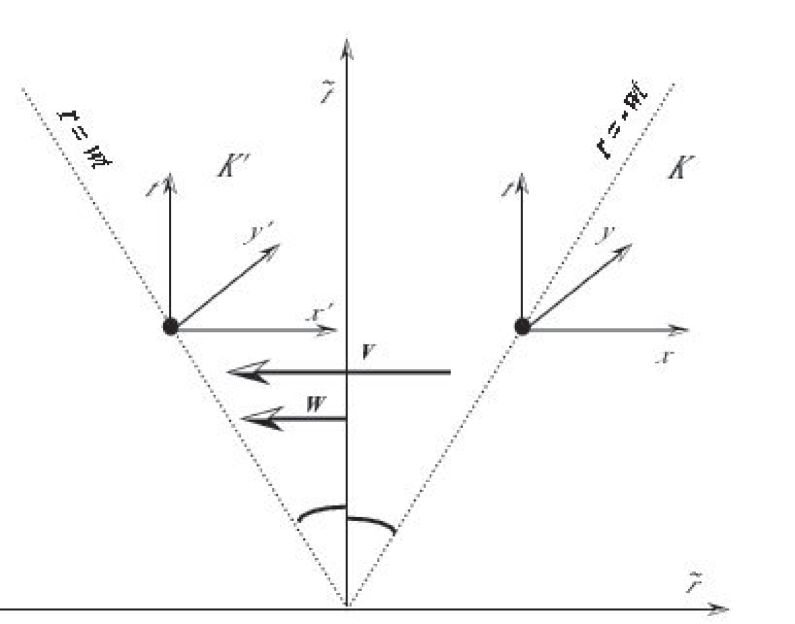
Figure 1: The physical meaning of symmetric velocity. Two inertial systems $K$ and $K^{\prime}$ with relative velocity $\mathbf{v}$ between them are viewed from the system connected to their center. In this system, $K$ and $K^{\prime}$ are each moving with velocity $\pm\mathbf{w}$.

Instead of $\mathbf{w_{s}}$, we shall find it more convenient to use the unit-free vector $\mathbf{w}=\mathbf{w_{s}}/c$, which we call the s-velocity. The relation of a velocity $\mathbf{v}$ to its corresponding s-velocity is

$$\mathbf{v}=\Phi(\mathbf{w})=\frac{2c\mathbf{w}}{1+|\mathbf{w}|^{2}},$$ (14)

where $\Phi$ denotes the function mapping the s-velocity $\mathbf{w}$ to its corresponding velocity $\mathbf{v}$. The s-velocity has some interesting and useful mathematical properties. The set of all three-dimensional relativistically admissible s-velocities forms a unit ball

$$D_{s}=\{\mathbf{w}\in R^{3}:\;|\mathbf{w}|<1\}.$$ (15)

Corresponding to the Einstein velocity addition equation, we may define an addition of s-velocities in $D_{s}$ such that

$$\Phi(\mathbf{b}\oplus_{s}\mathbf{w})=\Phi(\mathbf{b})\oplus_{E}\Phi(\mathbf{w}).$$ (16)

A straightforward calculation leads to the corresponding equation for s-velocity addition:

$$\mathbf{b}\oplus_{s}\mathbf{w}=\frac{(1+|\mathbf{w}|^{2}+2<\mathbf{b}\mid\mathbf{w}>)\mathbf{b}+(1-|\mathbf{b}|^{2})\mathbf{w}}{1+|\mathbf{b}|^{2}|\mathbf{w}|^{2}+2<\mathbf{b}\mid\mathbf{w}>}.$$ (17)

Equation (17) can be put into a more convenient form if, for any $\mathbf{b}\in D_{s}$, we define a map $\Psi_{\mathbf{b}}:D_{s}\to D_{s}$ by

$$\psi_{\mathbf{b}}(\mathbf{w})\equiv\mathbf{b}\oplus_{s}\mathbf{w}.$$ (18)

This map is an extension to $D_{s}\in R^{n}$ of the Möbius addition on the complex unit disc. It defines a conformal map on $D_{s}$. The motion of a charge in $\mathbf{E}\times\mathbf{B}$ fields is two-dimensional if the charge starts in the plane perpendicular to $\mathbf{B}$, and in this case Eq.(17) for s-velocity addition is somewhat simpler. By introducing a complex structure on the plane $\Pi$, which is perpendicular to $\mathbf{B}$, the disk $\Delta=D_{s}\cap\Pi$ can be identified as a unit disc $|w|<1$ called the Poincaré disc. In this case the s-velocity addition defined by Eq.(17) becomes

$$a\oplus_{s}w=\psi_{{a}}({w})=\frac{a+w}{1+\overline{a}w},$$ (19)

which is the well-known Möbius transformation of the unit disk.

By using the $s$ velocity we can rewrite ( as in [2]) the relativistic Lorentz force equation

$$\frac{d}{dt}(\gamma m\mathbf{v})=q({\bf E}+\mathbf{v}\times{\bf B})$$

as

$$\frac{m_{0}c}{q}\,\frac{d\mathbf{w}}{d\tau}=\left(\frac{1+|\mathbf{w}|^{2}}{2}\right){\bf{E}}+c\mathbf{w}\times{\bf{B}}-\mathbf{w}<\mathbf{w}|{\bf{E}}>,$$ (20)

which is the relativistic Lorentz force equation for the s-velocity $\mathbf{w}$ as a function of the proper time $\tau$.

We now use Eq.(20) to find the s-velocity of a charge $q$ in uniform, constant, and mutually perpendicular electric and magnetic fields. Since all of the terms on the right hand side of Eq. (20) are in the plane perpendicular to ${\mathbf{B}}$, if $\mathbf{w}$ is in the plane $\Pi$ perpendicular to ${\mathbf{B}}$, then $d{\mathbf{w}}/{d\tau}$ is also in $\Pi$. Consequently, if the initial s-velocity is in the plane perpendicular to ${\mathbf{B}}$, ${\mathbf{w}}$ will remain in the this plane and the motion will be two dimensional.

Working in Cartesian coordinates, we choose

$$\mathbf{E}=(0,E,0),\;\mathbf{B}=(0,0,B),\;\mbox{and}\;\mathbf{w}=(w_{1},w_{2},0).$$ (21)

By introducing a complex structure in $\Pi$ by denoting $w=w_{1}+iw_{2}$ the evolution equation Eq.(20) get the following simple form:

$$\frac{dw}{d\tau}=i\Omega\left(w^{2}-2\widetilde{B}w+1\right),$$ (22)

where

$$\Omega\equiv\frac{qE}{2m_{0}c}\;\;\mbox{and}\;\;\widetilde{B}\equiv\frac{cB}{E}.$$ (23)

The solution of Eq.(22) is unique for a given initial condition

$$w(0)=w_{0},$$ (24)

where the complex number $w_{0}$ represents the initial s-velocity $\mathbf{w}_{0}=\Phi^{-1}(\mathbf{v}_{0})$ of the charge.

Integrating Eq.(22) produces the equation

$$\int\frac{dw}{w^{2}-2\widetilde{B}w+1}=i\Omega\tau+C,$$ (25)

where the constant $C$ is determined from the initial condition (24). The way we evaluate this integral depends upon the sign of the discriminant $4\widetilde{B}^{2}-4$ associated with the denominator of the integrand. If we define

$$\Delta\equiv\widetilde{B}^{2}-1=\frac{(cB)^{2}-E^{2}}{E^{2}},$$ (26)

then the three cases $E<cB,E=cB\;\mbox{and}\;E>cB$ correspond to the cases $\Delta$ greater than zero, equal to zero, and less than zero.

Case 1 Consider first the case

$$\Delta=((cB)^{2}-{E}^{2})/{E}^{2})>0\Longleftrightarrow{E}<cB\;\mbox{and}\;\widetilde{B}>1.$$ (27)

The denominator of the integrand in (25) can be rewritten as

$$w^{2}-2\widetilde{B}w+1=(w-\alpha_{1})(w-\alpha_{2}),$$ (28)

where $\alpha_{1}$ and $\alpha_{2}$ are the real, positive roots

$$\alpha_{1}=\widetilde{B}-\sqrt{\widetilde{B}^{2}-1}\;\;\mbox{and}\;\;\alpha_{2}=\widetilde{B}+\sqrt{\widetilde{B}^{2}-1}.$$ (29)

and the solution then becomes:

$$w(\tau)=\frac{\alpha_{1}+Ce^{-i\nu\tau}}{1+\alpha_{1}Ce^{-i\nu\tau}}=\alpha_{1}\oplus_{s}Ce^{-i\nu\tau},$$ (30)

with

$$\nu=\left(\frac{q}{mc}\right)\sqrt{E^{2}-(cB)^{2}}.$$ (31)

This equation shows that in a system K’ moving with s-velocity $\alpha_{1}$ relative to the lab, the s-velocity of the charge corresponds to circular motion with initial s-velocity

$$C=\psi_{-\alpha_{1}}(w_{0}).$$ (32)

The s-velocity observed in K is shown in Figure 2.

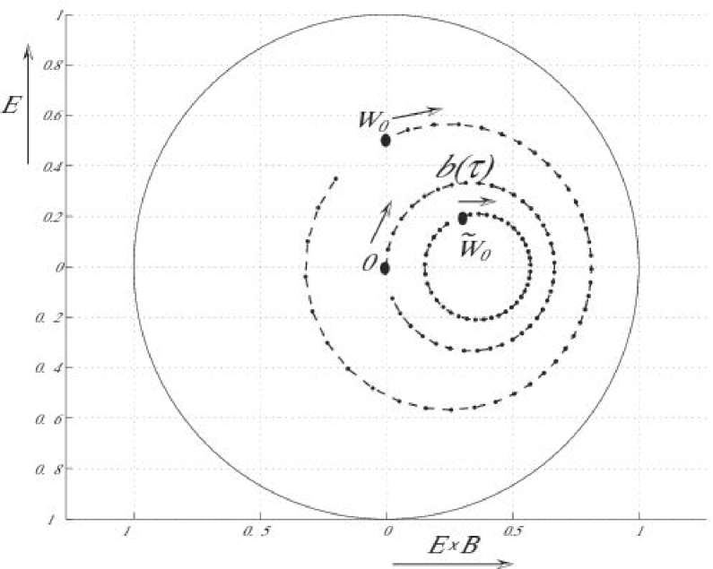
Figure 2: The trajectories of the s-velocity $w(\tau)$ of a charged particle with $q/m=10^{7}$C/kg in a constant uniform fields $E=1$V/m and $cB=1.5$V/m. The initial conditions are $w_{0}=-0.02+i0.5$ for the first trajectory and $\widetilde{w}_{0}=0.3+i0.2$ for the second. We also draw $b(\tau)$ corresponding to $w_{0}=0$. Note that all the trajectories are circles.

From Eqs.(14) and (29) it follows that the velocity corresponding to s-velocity $\alpha_{1}$ is

$$\frac{2c\alpha_{1}}{1+|\alpha_{1}|^{2}}=(E/B)\mathbf{i}=\mathbf{v}_{d}=v_{d}\mathbf{i},$$ (33)

which is the well-known $\mathbf{E}\times\mathbf{B}$ drift velocity. Applying the map $\Phi$ defined in Eq.(16) to both sides of (30), we get

$$\mathbf{v}(\tau)=\mathbf{v}_{d}\oplus_{E}e^{-i\nu\tau}\Phi(C).$$ (34)

Eq.(34) says that the total velocity of the charge, as a function of the proper time, is the sum of a constant drift velocity $\mathbf{v}_{d}=(E/B)\mathbf{i}$ and circular motion, as expected.

If we let

$$\Phi(C)=|\Phi(C)|e^{i\tau_{0}}=\widetilde{v}_{0}e^{i\tau_{0}},$$ (35)

then the velocity of the charge is

$$\mathbf{v}(\tau)=\mathbf{v}_{d}\oplus_{E}\widetilde{v}_{0}e^{-i\nu(\tau-\tau_{0})}.$$ (36)

The position of the charge as a function of the proper time is

$$\mathbf{r}(\tau)=\int_{0}^{\tau}\gamma\mathbf{v}(\tau^{\prime})\,d\tau^{\prime}=\frac{\gamma_{d}v_{d}}{\nu}\left(\gamma_{d}(\nu\tau-\sin{\nu\tau}),(\cos\nu\tau-1)\right)$$ (37)

and the lab time $t$ as a function of the proper time is

$$t(\tau)=\int_{0}^{\tau}\gamma(\tau^{\prime})d\tau^{\prime}=\frac{\gamma_{d}^{2}}{\nu}\left(\nu\tau-\frac{v_{d}^{2}}{c^{2}}\sin{\nu\tau}\right),$$ (38)

where $\gamma_{d}=\gamma(\mathbf{v}_{d})$. The world line $\mathbf{r}(\tau),t(\tau)$ of such test particle is presented on Figure 3.

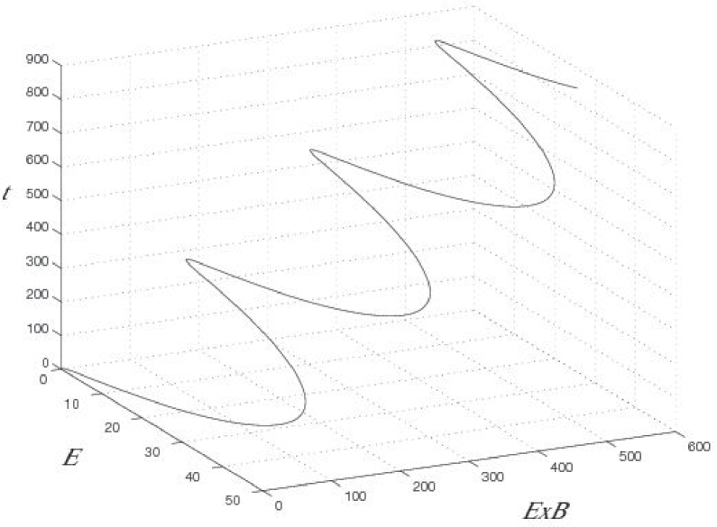
Figure 3: The world line $\mathbf{r}(\tau),t(\tau)$ of the test particle of Figure 2 in the same electromagnetic field. The initial velocity $\mathbf{v}_{0}=(0,0,0)$.

Case 2  Next consider the case $\Delta=((cB)^{2}-{E}^{2})/{E}^{2}=0\Longleftrightarrow{E}=c{B}\;\mbox{and}\;\widetilde{B}=1$. The denominator in the integrand of (25) is $w^{2}-2w+1=(w-1)^{2}$ and its solution is

$$w(\tau)=1-\frac{1}{i\Omega\tau+C}$$ (39)

with $C=-\frac{1}{w_{0}-1}.$ This s-velocity is graphed in Figure 4.

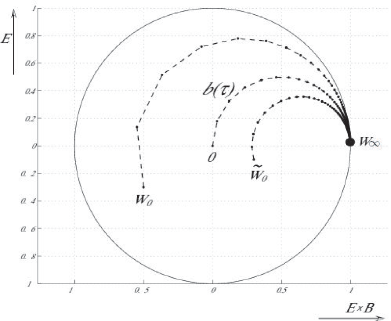
Figure 4: The trajectories of the s-velocity $w(\tau)$ of a charged particle with $q/m=10^{7}$C/kg in constant, uniform fields $E=1$V/m and $cB=1$V/m. The initial conditions are $w_{0}=-0.5-i0.3$ and $\widetilde{w}_{0}=0.3-i0.1$. Also shown is $b(\tau)$, corresponding to $w_{0}=0$. Note that each trajectory is a circular arc and that they all end at $w_{\infty}=1.$

If the initial velocity is zero, $C=1$ and using that $\gamma\mathbf{v}=\frac{2c\mathbf{w}}{1-|\mathbf{w}|^{2}},$ the position of the charge as a function of the proper time is

$$\mathbf{r}(\tau)=2c\left(\frac{\Omega^{2}\tau^{3}}{3},\frac{\Omega\tau^{2}}{2}\right).$$ (40)

and the lab time as a function of the proper time is

$$t(\tau)=\int_{0}^{\tau}\gamma(\tau^{\prime})d\tau^{\prime}=\tau+\frac{2\Omega^{2}}{3}\tau^{3}.$$ (41)

Equations (40) and (41) give the complete solution for this case. The space trajectories $\mathbf{r}(t)$ of the test particles is given on of Figure 5

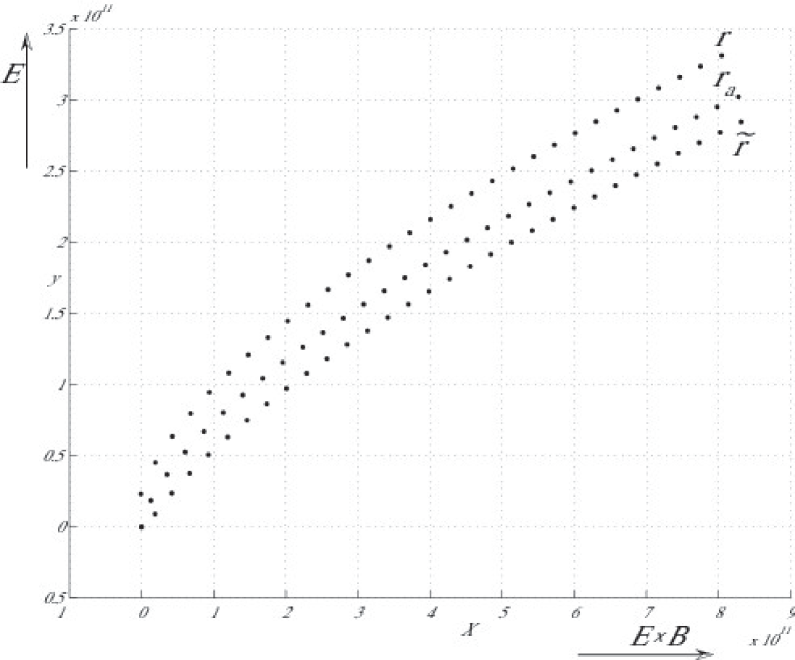
Figure 5: The space trajectories $\mathbf{r}(t)$ of the test particles of Figure 4 during 3000 seconds. The position of each particle is shown at fixed time intervals $dt=100s$.

Case 3  Consider the case $\Delta=((cB)^{2}-E^{2})/{E}^{2}<0\;\Longleftrightarrow{E}>cB\;\mbox{or}\;\widetilde{B}<1$.

Just as in Case 1, we rewrite the denominator of the integrand in Eq. (25) as $w^{2}-2\widetilde{B}w+1=(w-\alpha_{1})(w-\alpha_{2}),$ where

$$\alpha_{1}=\widetilde{B}-i\delta\;\;\mbox{and}\;\;\alpha_{2}=\widetilde{B}+i\delta=\overline{\alpha}_{1}$$ (42)

and $\delta=\sqrt{1-\widetilde{B}^{2}}>0.$ By introducing $\nu$ as in (31) and an s-velocity ${w}_{d}\equiv{\widetilde{B}}/\left({1+\delta}\right)$ we can write the solution as:

$$w(\tau)=w_{d}\oplus_{s}(i\tanh(\nu\tau)\oplus_{s}\widetilde{w}_{0}).$$ (43)

This s-velocity is graphed in Figure 6

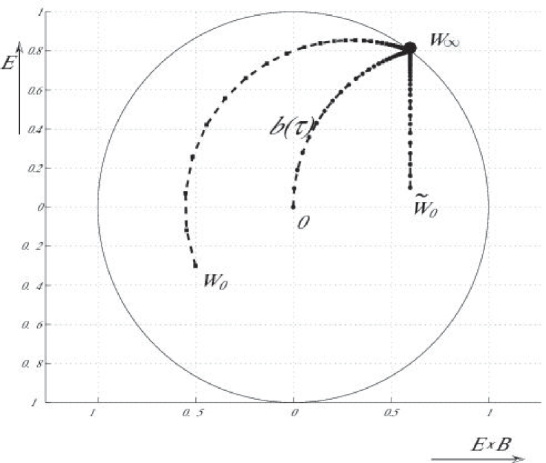
Figure 6: The trajectories of the s-velocity $w(\tau)$ of a charged particle with $q/m=10^{7}$C/kg in constant, uniform fields ${\bf E}=1$V/m and $cB=0.6$V/m. The initial conditions are $w_{0}=-0.5-i0.3$ and $\widetilde{w}_{0}=0.6+i0.1$. Also shown is $b(\tau)$, corresponding to $w_{0}=0$. Note that the trajectories all end at $w_{\infty}=0.6+i0.8$.

For the velocity of the charge we get

$$\mathbf{v}(\tau)=\mathbf{v}_{d}\oplus_{E}(c\tanh(2\nu\tau)\mathbf{j}\oplus\widetilde{\mathbf{v}}_{0}),$$ (44)

where $\mathbf{v}_{d}=(c^{2}B/E)\mathbf{i}$ is the drift velocity and $\widetilde{\mathbf{v}}_{0}$ is the initial velocity in the drift frame. From this it follows that

$$\mathbf{r}(\tau)=\int_{0}^{\tau}\gamma\mathbf{v}(\tau^{\prime})\,d\tau^{\prime}=\frac{\gamma_{d}}{\nu^{\prime}}\left(\gamma_{d}v_{d}(\sinh(\nu^{\prime}\tau)-\nu^{\prime}\tau),c(\cosh(\nu^{\prime}\tau)-1)\right)$$ (45)

and the lab time $t$ as a function of the proper time is

$$t(\tau)=\int_{0}^{\tau}\gamma(\tau^{\prime})d\tau^{\prime}=\gamma_{d}^{2}\left(\frac{\sinh(\nu^{\prime}\tau)}{\nu^{\prime}}-\frac{v_{d}^{2}}{c^{2}}\tau\right).$$ (46)

Equations (45) and (46) together give the complete solution for this case. The space trajectory is given in Figure 7.

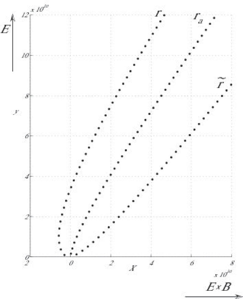
Figure 7: The space trajectories $\mathbf{r}(t)$ of the test particles of Figure 6 in the same electromagnetic field during 500 seconds. The position of each particle is shown at fixed time intervals $dt=10s$.

5 Relativistic Dynamics of the four-velocity

In this section we will use four-velocity instead of velocity to describe the relativistic evolution.

To define the four velocity, we consider the Lorentz space-time transformation between two inertial systems $K^{\prime}$ and $K$ with axes chosen to be parallel. We assume that $K^{\prime}$ moves with respect to $K$ with relative velocity $\mathbf{b}$. In order for all the coordinates to have the same units, we describe an event in $K^{\prime}$ by $\begin{pmatrix}ct^{\prime}\\ \mathbf{r}^{\prime}\end{pmatrix}$ and by $\begin{pmatrix}ct\\ \mathbf{r}\end{pmatrix}$ in $K$. The Lorentz transformation can be now written as in formula (19) of Part 1 as

$$\left(\begin{array}[]{c}ct\\ \mathbf{r}\end{array}\right)=L_{\mathbf{b}}\left(\begin{array}[]{c}ct^{\prime}\\ \mathbf{r}^{\prime}\end{array}\right)=\gamma\left(\begin{array}[]{cc}1&\frac{\mathbf{b}^{T}}{c}\\ \frac{\mathbf{b}}{c}&P_{\mathbf{b}}+\gamma^{-1}(I-P_{\mathbf{b}})\end{array}\right)\left(\begin{array}[]{c}ct^{\prime}\\ \mathbf{r}^{\prime}\end{array}\right),$$ (47)

with $\gamma=\gamma(\mathbf{b})=1/\sqrt{1-|\mathbf{b}|^{2}/c^{2}}$.

Consider now the space-time evolution of the origin $O^{\prime}$ of system $K^{\prime}$. This origin has space coordinate $\mathbf{r}^{\prime}=0$ and thus by (47) its evolution in $K$ is given by

$$\left(\begin{array}[]{c}ct\\ \mathbf{r}\end{array}\right)=\gamma(\mathbf{b})\left(\begin{array}[]{c}c\\ \mathbf{b}\end{array}\right)t^{\prime}.$$ (48)

This shows that $O^{\prime}$ moves with uniform proper velocity $\gamma(\mathbf{b})\left(\begin{array}[]{c}c\\ \mathbf{b}\end{array}\right)$ in $K$, which is called the four-velocity corresponding to $\mathbf{b}$, which we will denote by $\tilde{b}$. In other words

$$\tilde{b}=\gamma(\mathbf{b})\left(\begin{array}[]{c}c\\ \mathbf{b}\end{array}\right),$$ (49)

which is a four-dimensional vector. The four-velocity expresses not only the change of the position of an object but also the change of the time rate of the clock comoving with the object.

Here too, we will assume the $EP^{2}$ principle, which implies that the acceleration of an object under a given force in an inertial system $K$ is equivalent to free motion in system $K^{\prime}$ moving with a variable relative velocity $\mathbf{b}(t)$ with respect to $K$. Also here we may assume that $\mathbf{b}(0)=0.$ Denote the initial velocity of the object in $K^{\prime}$ by $\mathbf{v}$. Since the motion of the object in system $K^{\prime}$ is free, the velocity of the object will remain constant in $K^{\prime}$. The four-velocity $\tilde{v}=\gamma(\mathbf{v})\left(\begin{array}[]{c}c\\ \mathbf{v}\end{array}\right)$ will also remain constant. We denote the proper time of the object by $\tau$. By use of (47) and (48) and the well-known formulas (see [2]) for relativistic velocity addition and the transformation of the corresponding $\gamma$’s, we can calculate the world-line of the the object in $K$ as

$$\left(\begin{array}[]{c}ct\\ \mathbf{r}\end{array}\right)=L_{\mathbf{b}}\left(\begin{array}[]{c}ct^{\prime}\\ \mathbf{r}^{\prime}\end{array}\right)=L_{\mathbf{b}(t)}\tilde{v}\tau=L_{\mathbf{b}}\gamma(\mathbf{v})\left(\begin{array}[]{c}c\\ \mathbf{v}\end{array}\right)\tau=$$

$$=\gamma(\mathbf{b})\gamma(\mathbf{v})\left(\begin{array}[]{cc}1&\frac{\mathbf{b}^{T}}{c}\\ \frac{\mathbf{b}}{c}&P_{\mathbf{b}}+\gamma(\mathbf{b})^{-1}(I-P_{\mathbf{b}})\end{array}\right)\left(\begin{array}[]{c}c\\ \mathbf{v}\end{array}\right)\tau=$$

$$=\gamma(\mathbf{b})\gamma(\mathbf{v})\left(\begin{array}[]{c}c+\frac{\mathbf{b}\cdot\mathbf{v}}{c}\\ \mathbf{b}+P_{\mathbf{b}}+\gamma(\mathbf{b})^{-1}(I-P_{\mathbf{b}})\end{array}\right)\tau=$$

$$=\gamma(\mathbf{b})\gamma(\mathbf{v})(1+\frac{\mathbf{b}\cdot\mathbf{v}}{c^{2}})\left(\begin{array}[]{c}c\\ \mathbf{b}\oplus\mathbf{v}\end{array}\right)\tau=\gamma(\mathbf{b}\oplus\mathbf{v})\left(\begin{array}[]{c}c\\ \mathbf{b}\oplus\mathbf{v}\end{array}\right)\tau.$$ (50)

This shows that $L_{\mathbf{b}(t)}\tilde{v}=\widetilde{\mathbf{b}\oplus\mathbf{v}}$ and that the four velocity transformation between $K^{\prime}$ and $K$ is given by multiplication by the $4\times 4$ matrix of $L_{\mathbf{b}}$.

As a result, the relativistic acceleration, which is the generator of the four-velocity changes, is obtained by differentiating the matrix of $L_{\mathbf{b}(t)}$ with respect to $t$ at $t=0$. Since $\mathbf{b}(0)=0$, we have $\gamma(\mathbf{b}(0))=1$ and $\frac{d}{dt}\gamma(\mathbf{b}(t))\Bigr{|}_{t=0}=0$, Denoting $\frac{d}{dt}\mathbf{b}(t)\Bigr{|}_{t=0}=\mathbf{a},$ we get the matrix for relativistic acceleration

$$\delta(L_{\mathbf{b}(t)})=\frac{d}{dt}L_{\mathbf{b}(t)}\Bigr{|}_{t=0}=\frac{1}{c}\left(\begin{array}[]{cc}0&\mathbf{a}^{T}\\ \mathbf{a}&0\end{array}\right).$$ (51)

Using the fact that for small velocities $\mathbf{f}=m_{0}\mathbf{a}$, by Newton’s dynamic law, the four-velocity and relativistic acceleration in special relativity become:

$$m_{0}\frac{1}{c}\left(\begin{array}[]{cc}0&\mathbf{a}^{T}\\ \mathbf{a}&0\end{array}\right)\gamma(\mathbf{v})\left(\begin{array}[]{c}c\\ \mathbf{v}\end{array}\right)=m_{0}\gamma(\mathbf{v})\left(\begin{array}[]{c}\frac{\mathbf{a}\cdot\mathbf{v}}{c}\\ \mathbf{a}\end{array}\right)=\gamma(\mathbf{v})\left(\begin{array}[]{c}\frac{\mathbf{f}\cdot\mathbf{v}}{c}\\ \mathbf{f}\end{array}\right).$$ (52)

The last expression is called the four-force, see [5] p. 123.

General four-velocity transformations between two inertial systems also include rotations, which can be expressed by a $3\times 3$ orthogonal matrices $U(t)$. We will extend such a matrix to a $4\times 4$ matrix by adding zeros in the time components outside the diagonal and assume that $T(0)=I$. The general four-velocity transformation will then be

$$T(t)=L_{\mathbf{b}(t)}U(t)$$ (53)

and its generator, representing relativistic acceleration, is

$$\delta(T(t))=\frac{d}{dt}T(t)\Bigr{|}_{t=0}=\frac{d}{dt}L_{\mathbf{b}(t)}\Bigr{|}_{t=0}+\frac{d}{dt}U(t)\Bigr{|}_{t=0}=\frac{1}{c}\left(\begin{array}[]{cc}0&\mathbf{a}^{T}\\ \mathbf{a}&A\end{array}\right),$$ (54)

where $A=\frac{d}{dt}T(t)\Bigr{|}_{t=0}$ is a $3\times 3$ antisymmetric matrix.

We have seen that relativistic acceleration includes both linear and rotational acceleration and is a linear map on the four-velocities. The matrix representing the relativistic acceleration is antisymmetric if both indices are space indices or both are time indices and is symmetric if one of the indices is spacial and the other is a temporal. Moreover, any relativistic force, which is a multiple of the relativistic acceleration by $m_{0}$, must have the form of the electromagnetic tensor

$$\hat{F}=\frac{q}{c}\left(\begin{array}[]{cccc}0&E_{1}&E_{2}&E_{3}\\ E_{1}&0&B_{3}&-B_{2}\\ E_{2}&-B_{3}&0&B_{1}\\ E_{3}&B_{2}&-B_{1}&0\end{array}\right)$$ (55)

and must transform from one inertial system to another in the same way that this tensor transforms. The electromagnetic dynamic equation in our notation is

$$m_{0}\frac{d}{d\tau}\tilde{v}=\hat{F}\tilde{v}.$$ (56)

In classical mechanics, a force was represented by a differential one-form which expressed the change of the velocity and space displacement of the object in the direction of the force. In special relativity, a force (a non-rotating one) causes more change then it causes in classical mechanics. It also causes a change in the rate of a clock connected to the object due to the change of the magnitude of the object’s velocity. Thus, it has to be represented by a differential two-form. On the other hand, forces causing rotation, like the magnetic force need to be described by differential two-forms also in classical mechanics. Thus, only in relativistic dynamics can these two forces be combined effectively as a single force.

6 Discussion

We have shown that an analog of the Equivalence Principle leads to the known relativistic dynamic equation. The relativistic force is defined by an element of the Lie algebra of the group $Aut_{p}(D_{v})$ of projective automorphisms of the ball of relativistically admissible velocities $D_{v}$. This Lie algebra is a quadratic polynomial on $D_{v}$ where the constant and quadratic coefficients define an analog of electric force, while the linear term corresponds to a magnetic force. Such decomposition exists for any force in relativity. The Lie algebra $aut_{p}(D_{v})$ is described by the triple product associated with the domain $D_{v}$ which is a domain of type I in Cartan’s classification.

The relativistic force on a new dynamic variable - symmetric velocity- is an element of $aut_{c}(D_{s})$- the Lie algebra of the conformal group on the ball of relativistically admissible symmetric velocities $D_{s}$. For velocities with the speed of light, the symmetric velocity and the regular velocity are equal. This explains the known fact that the Maxwell equations (related to electro-magnetic propagation with the speed of light) are invariant under the conformal group. But in order to obtain conformal transformation for massive particles we must use symmetric velocity instead of the regular velocity. The use of symmetric velocity helps to find analytic solutions for relativistic dynamic equations.

The Lie algebra $aut_{c}(D_{s})$ is described by the triple product associated with the domain $D_{s}$. In this case, this is a domain of type IV in Cartan’s classification, called the Spin factor. A complexification of this domain leads to Dirac bispinors, an analog of the geometric product of Clifford algebras. We also obtain both spin 1 and spin $1/2$ representations of the Lorentz group on this domain, see [3]. This may provide a connection between Relativity and Quantum Mechanics.

By applying the analog of the Equivalence Principle to the four-velocity we showed that the relativistic dynamics equation leads to an analog of the electro-magnetic tensor.

We want to thank Dr. Tzvi Scaar and Michael Danziger for helpful remarks.

References

- [1] W. E. Baylis, Electrodynamics, A Modern Geometric Approach, Progress in Physics 17, Birkhäuser, Boston, (1999).
- [2] Y. Friedman, Physical Applications of Homogeneous Balls, Progress in Mathematical Physics 40 Birkhäuser, Boston, (2004).
- [3] Y. Friedman,Geometric tri-product of the spin domain and Clifford algebras, to appear in the proceedings of 7th International Congress of Clifford Algeras, http:// arxiv.org/abs/math-ph/0510008
- [4] Y. Friedman, M.Semon, Relativistic acceleration of charged particles in uniform and mutually perpendicular electric and magnetic fields as viewed in the laboratory frame, Phys. Rev. E 72 (2005), 026603.
- [5] W. Rindler, Relativity: Special, General and Cosmological, Oxford University press (2004)
- [6] G. Scarpetta, Lett. Nuovo Cimento 41 (1984) 51.
- [7] S. Takeuchi, Phys. Rev. E66, 37402-1 (2002).