Understanding d’Alembert’s principle: System of Pendulums

Abstract

Lagrangian mechanics uses d’Alembert’s principle of zero virtual work as an important starting point. The orthogonality of the force of constraint and virtual displacement is emphasized in literature, without a clear warning that this is true usually for a single particle system. For a system of particles connected by constraints, it is shown, that the virtual work of the entire system is zero, even though the virtual displacements of the particles are not perpendicular to the respective constraint forces. It is also demonstrated why d’Alembert’s principle involves virtual work rather than the work done by constraint forces on allowed displacements.

I Introduction

The principle of zero work by constraint forces on virtual displacement, also known as d’Alembert’s principle, is an important step in formulating and solving a mechanical problem with constraints goldstein ; greenwood ; hylleraas ; sommer ; taylor . In the simple systems widely used in literature, e.g., a single particle rolling down a frictionless incline, or a simple pendulum with inextensible ideal string, the force of constraint is perpendicular to the virtual displacement. This results in zero virtual work by constraint forces. It is often tempting to assume that the constraint forces are always orthogonal to respective virtual displacements, even for a system of particles. d’Alembert’s principle then seems to be a consequence of this orthogonality goldstein ; hylleraas ; taylor .

In this article we study two simple systems: a double pendulum and an $N$-pendulum. In these systems it is observed that, the virtual displacements are not perpendicular to the respective constraint forces acting on individual particles (pendulum bobs). However, d’Alembert’s principle of zero virtual work still holds for the systems as a whole. In these problems, the principle of zero virtual work is a consequence of, (i) the relation between the virtual displacements of coupled components (neighbouring bobs), and (ii) the appearance of (Newtonian) action-reaction pairs in forces of constraint between neighbouring particles. Thus d’Alembert’s principle is more subtle and involved than it is often thought to be. Greenwood has rightly said, “… workless constraints do no work on the system as a whole in an arbitrary virtual displacement. Quite possibly, however, the workless constraint forces will do work on individual particles of the system” greenwood .

II Double Pendulum

Let us first consider a double pendulum, with inextensible ideal strings of lengths $L_{1}$ and $L_{2}$. Let $\mathbf{r}_{1}$ and $\mathbf{r}_{2}$ denote the instantaneous positions of the pendulum bobs $\mathcal{P}_{1}$ and $\mathcal{P}_{2}$, with respect to the point of suspension (see figure 1). When the system is suspended from a stationary support; the holonomic, scleronomous constraint equations are,

$$|\mathbf{r}_{1}|=L_{1},\hskip 28.45274pt|\mathbf{r}_{1}-\mathbf{r}_{2}|=L_{2}.$$ (1)

The equations for allowed velocities are obtained by differentiating (1) with respect to $t$,

$$\mathbf{r}_{1}\cdot\mathbf{v}_{1}=0,\hskip 28.45274pt(\mathbf{r}_{2}-\mathbf{r}_{1})\cdot(\mathbf{v}_{2}-\mathbf{v}_{1})=0.$$ (2)

Thus, the allowed velocity $\mathbf{v}_{1}$ of $\mathcal{P}_{1}$ is orthogonal to its position vector $\mathbf{r}_{1}$. The relative velocity of the second bob $(\mathbf{v}_{2}-\mathbf{v}_{1})$ with respect to the first, is orthogonal to the relative position vector $\mathbf{r}_{21}=(\mathbf{r}_{2}-\mathbf{r}_{1})$. Let $\hat{\mathbf{n}}_{1}$ and $\hat{\mathbf{n}}_{2}$ be unit vectors orthogonal to ($\mathbf{r}_{1}$) and ($\mathbf{r}_{2}-\mathbf{r}_{1}$) respectively,

$$\hat{\mathbf{n}}_{1}\cdot\mathbf{r}_{1}=0\hskip 28.45274pt\mbox{and}\hskip 28.45274pt\hat{\mathbf{n}}_{2}\cdot(\mathbf{r}_{2}-\mathbf{r}_{1})=0.$$ (3)

From (2) and (3) we obtain the allowed velocities as,

$$\mathbf{v}_{1}=b_{1}\hat{\mathbf{n}}_{1},\hskip 28.45274pt\mathbf{v}_{2}-\mathbf{v}_{1}=b_{2}\hat{\mathbf{n}}_{2}\hskip 14.22636pt\Rightarrow\hskip 14.22636pt\mathbf{v}_{2}=\mathbf{v}_{1}+b_{2}\hat{\mathbf{n}}_{2}$$ (4)

where $b_{1}$ and $b_{2}$ are arbitrary real constants, denoting the magnitude of the relevant vectors.

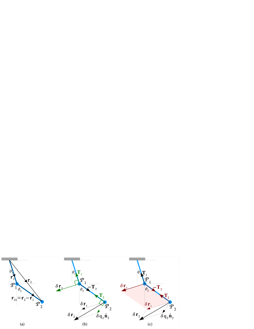
Figure 1: Double pendulum: (a) position vectors, (b) orthogonality of tensions to part of virtual displacements, (c) cancellation of part of virtual work related to action-reaction pair (tension)

The virtual velocities are defined as a difference between two allowed velocities, $\widetilde{\mathbf{v}}_{k}=\mathbf{v}_{k}-\mathbf{v}_{k}^{\prime}$ sj_ejp_27 . The allowed displacements $d\mathbf{r}_{k}$, and the virtual displacements $\delta\mathbf{r}_{k}$ are then given by,

$$d\mathbf{r}_{1}=\mathbf{v}_{1}\,dt=dq_{1}\hat{\mathbf{n}}_{1},$$

$$\delta\mathbf{r}_{1}=d\mathbf{r}_{1}-d\mathbf{r}_{1}^{\prime}=(dq_{1}-dq_{1}^{\prime})\hat{\mathbf{n}}_{1}=\delta q_{1}\hat{\mathbf{n}}_{1}.$$ (5)

$$d\mathbf{r}_{2}=\mathbf{v}_{2}dt=\mathbf{v}_{1}dt+b_{2}\hat{\mathbf{n}}_{2}dt=d\mathbf{r}_{1}+dq_{2}\hat{\mathbf{n}}_{2},$$

$$\delta\mathbf{r}_{2}=(d\mathbf{r}_{1}+dq_{2}\hat{\mathbf{n}}_{2})-(d\mathbf{r}_{1}^{\prime}++dq_{2}^{\prime}\hat{\mathbf{n}}_{2})=\delta\mathbf{r}_{1}+\delta q_{2}\hat{\mathbf{n}}_{2}.$$ (6)

It may be noted that, under the given holonomic, scleronomous constraints (velocity and time independent), the sets of allowed and virtual displacements are equivalent.

A set of allowed displacements $\{d\mathbf{r}_{1},d\mathbf{r}_{2}\}$ is obtained by a specific choice of the numbers $\{b_{1},b_{2}\}$ or $\{dq_{1},dq_{2}\}$. By making different choices of the set $\{dq_{1},dq_{2}\}$ we get a whole family of allowed displacements, $\{d\mathbf{r}_{k}\}$, where,

$$\{d\mathbf{r}_{k}\}\Rightarrow\{d\mathbf{r}_{1},d\mathbf{r}_{2}\}_{\{b_{1},b_{2}\}}=\{d\mathbf{r}_{1},d\mathbf{r}_{2}\}_{\{dq_{1},dq_{2}\}}.$$

Or more precisely,

$$\{d\mathbf{r}_{k}\}\Rightarrow\{\{d\mathbf{r}_{1},d\mathbf{r}_{2}\}_{\{b_{1},b_{2}\}}|b_{1},b_{2}\in\Re\}$$

where $\Re$ is the set of real numbers. Similarly, by choosing different set of quantities $\{\delta q_{1},\delta q_{2}\}$ we get the family of virtual displacements, $\{\delta\mathbf{r}_{k}\}$, where,

$$\{\delta\mathbf{r}_{k}\}\Rightarrow\{\delta\mathbf{r}_{1},\delta\mathbf{r}_{2}\}_{\{\delta q_{1},\delta q_{2}\}}.$$

Thus, it is easy to see that for holonomic, scleronomous constraints, the set of all possible allowed displacements is the same as the set of all possible virtual displacements. This is in agreement with the fact that for holonomic, scleronomous systems, the sets $\{d\mathbf{r}_{k}\}$ and $\{\delta\mathbf{r}_{k}\}$ satisfy the same equationssj_ejp_eqn , namely,

$$\begin{array}[]{l l}\mathbf{r}_{1}\cdot d\mathbf{r}_{1}=0,&(\mathbf{r}_{2}-\mathbf{r}_{1})\cdot(d\mathbf{r}_{2}-d\mathbf{r}_{1})=0\\ \mathbf{r}_{1}\cdot\delta\mathbf{r}_{1}=0,&(\mathbf{r}_{2}-\mathbf{r}_{1})\cdot(\delta\mathbf{r}_{2}-\,\delta\mathbf{r}_{1})=0\\ \end{array}$$

As the pendulums are suspended by inextensible ideal strings, one may assume that the tensions in the strings act along their lengths. This essentially implies that there is no shear in the string to transmit transverse force. Thus the tension $\mathbf{T}_{1}$ is along $(-\mathbf{r}_{1})$ and tension $\mathbf{T}_{2}$ is along $(\mathbf{r}_{1}-\mathbf{r}_{2})$. Hence, the virtual displacement $\delta\mathbf{r}_{1}$ for the first pendulum is perpendicular to the tension $\mathbf{T}_{1}$, but the virtual displacement $\delta\mathbf{r}_{2}$ of the second pendulum is not perpendicular to $\mathbf{T}_{2}$.

$$\mathbf{T}_{1}\cdot\delta\mathbf{r}_{1} = 0$$

$$\mathbf{T}_{2}\cdot\delta\mathbf{r}_{2} = \mathbf{T}_{2}\cdot(\delta\mathbf{r}_{1}+\delta q_{2}{\hat{\mathbf{n}}}_{2})=\mathbf{T}_{2}\cdot\delta\mathbf{r}_{1}+(\mathbf{T}_{2}\cdot\hat{\mathbf{n}}_{2})\delta q_{2}=\mathbf{T}_{2}\cdot\delta\mathbf{r}_{1}$$ (7)

At this stage one may appreciate that $\mathbf{T}_{1}$ is not the entire force of constraint on $\mathcal{P}_{1}$. As a reaction to $\mathcal{P}_{1}$ pulling $\mathcal{P}_{2}$ with a tension $\mathbf{T}_{2}$, the second bob $\mathcal{P}_{2}$ pulls the first bob $\mathcal{P}_{1}$ with a tension $(-\mathbf{T}_{2})$. Thus the virtual work by constraint forces acting on $\mathcal{P}_{1}$ and $\mathcal{P}_{2}$ are given by,

$$\delta\mathcal{W}_{1}=\mathbf{R}_{1}\cdot\delta\mathbf{r}_{1}=(\mathbf{T}_{1}-\mathbf{T}_{2})\cdot\delta\mathbf{r}_{1}=-\mathbf{T}_{2}\cdot\delta\mathbf{r}_{1}\neq 0$$

$$\delta\mathcal{W}_{2}=\mathbf{R}_{2}\cdot\delta\mathbf{r}_{2}=\mathbf{T}_{2}\cdot(\delta\mathbf{r}_{1}+\delta q_{2}\hat{\mathbf{n}}_{2})=\mathbf{T}_{2}\cdot\delta\mathbf{r}_{1}\neq 0.$$ (8)

Although neither $\delta\mathcal{W}_{1}$ nor $\delta\mathcal{W}_{2}$ is zero, their sum adds up to zero. Thus the “equal and opposite” Newtonian reaction comes to our rescue, and we have a cancellation in the total virtual work.

$$\delta\mathcal{W}_{1}+\delta\mathcal{W}_{2}=\mathbf{R}_{1}\cdot\delta\mathbf{r}_{1}+\mathbf{R}_{2}\cdot\delta\mathbf{r}_{2}=-\mathbf{T}_{2}\cdot\delta\mathbf{r}_{1}+\mathbf{T}_{2}\cdot\delta\mathbf{r}_{1}=0$$ (9)

This shows that in the case of a double pendulum with stationary support, d’Alembert’s principle utilizes the equal and opposite nature of the tensions between neighbouring bobs (Newtonian action-reaction pair).

Let us now consider the double pendulum with a moving point of suspension. This gives us a system with a rheonomous constraint. Let the velocity of the point of suspension be $\mathbf{v}_{0}$. The constraint equations in this case are,

$$|\mathbf{r}_{1}-\mathbf{v}_{0}t|=L_{1},\hskip 28.45274pt|\mathbf{r}_{2}-\mathbf{r}_{1}|=L_{2}$$ (10)

The only non-trivial modification is that, the virtual displacements are no longer equivalent to the allowed displacements.

For the first bob $\mathcal{P}_{1}$,

$$d\mathbf{r}_{1}=\mathbf{v}_{1}\,dt=\mathbf{v}_{0}\,dt+dq_{1}\hat{\mathbf{n}}_{1},$$

$$\delta\mathbf{r}_{1}=d\mathbf{r}_{1}-d\mathbf{r}_{1}^{\prime}=(\mathbf{v}_{0}dt\hskip-17.07182pt\backslash\,\,\,\backslash\,+dq_{1}\hat{\mathbf{n}}_{1})-(\mathbf{v}_{0}dt\hskip-17.07182pt\backslash\,\,\,\backslash\,+dq_{1}^{\prime}\hat{\mathbf{n}}_{1})=(dq_{1}-dq_{1}^{\prime})\hat{\mathbf{n}}_{1}=\delta q_{1}\hat{\mathbf{n}}_{1}.$$ (11)

Therefore virtual displacement $\delta\mathbf{r}_{1}$ is a vector along $\hat{\mathbf{n}}_{1}$, whereas allowed displacement $d\mathbf{r}_{1}$ is sum of a vector along $\hat{\mathbf{n}}_{1}$ and a vector along $\mathbf{v}_{0}$. For the second bob $\mathcal{P}_{2}$,

$$d\mathbf{r}_{2}=\mathbf{v}_{2}dt=\mathbf{v}_{1}dt+b_{2}\hat{\mathbf{n}}_{2}dt=\mathbf{v}_{0}dt+dq_{1}\hat{\mathbf{n}}_{1}+dq_{2}\hat{\mathbf{n}}_{2}$$

$$\delta\mathbf{r}_{2}=(\mathbf{v}_{0}dt\hskip-17.07182pt\backslash\,\,\,\backslash\,+dq_{1}\hat{\mathbf{n}}_{1}+dq_{2}\hat{\mathbf{n}}_{2})-(\mathbf{v}_{0}dt\hskip-17.07182pt\backslash\,\,\,\backslash\,+dq_{1}^{\prime}\hat{\mathbf{n}}_{1}+dq_{2}^{\prime}\hat{\mathbf{n}}_{2})=\delta q_{1}\hat{\mathbf{n}}_{1}+\delta q_{2}\hat{\mathbf{n}}_{2}.$$ (12)

Thus $d\mathbf{r}_{1}$ and $d\mathbf{r}_{2}$ are not equivalent to $\delta\mathbf{r}_{1}$ and $\delta\mathbf{r}_{2}$. However the relation between $\delta\mathbf{r}_{1}$ and $\delta\mathbf{r}_{2}$ remains the same as in the case of a double pendulum with stationary support.

$$\delta\mathbf{r}_{2}=\delta\mathbf{r}_{1}+\delta q_{2}\hat{\mathbf{n}}_{2}$$ (13)

Hence the above inferences, in particular, (II), (II), (9) are true even in this case.

III N-Pendulum

It is instructive to repeat the above exercise for a system of $N$-pendulum joined end to end by inextensible, ideal strings. Let $\mathbf{r}_{1},\mathbf{r}_{2},\dots,\mathbf{r}_{N}$ denote the instantaneous position vectors of pendulum bobs $\mathcal{P}_{1},\mathcal{P}_{2},\dots,\mathcal{P}_{N}$ respectively, as shown in figure 2.

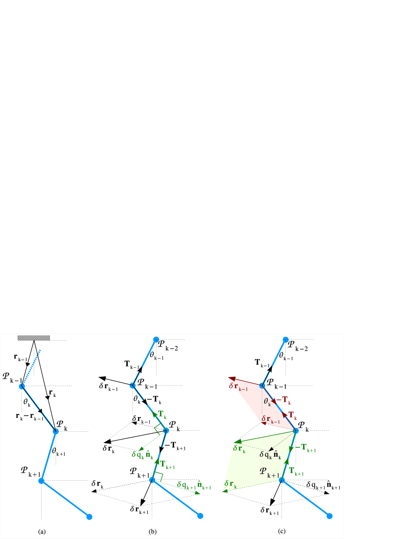
Figure 2: $N$-pendulum: (a) position vectors (position of the point of suspension in relation to the pendulum is schematic), (b) orthogonality of tensions to part of virtual displacements, (c) cancellation of part of virtual work related to action-reaction pair (tension)

The constraint equations for this system are,

$$|\mathbf{r}_{1}|=L_{1},\hskip 28.45274pt|\mathbf{r}_{k}-\mathbf{r}_{k-1}|=L_{k},\hskip 56.9055ptk=2,3,\dots,N.$$ (14)

The equations for allowed velocities, obtained by differentiating the above equations, are

$$\mathbf{r}_{1}\cdot\mathbf{v}_{1}=0,\hskip 28.45274pt(\mathbf{r}_{k}-\mathbf{r}_{k-1})\cdot(\mathbf{v}_{k}-\mathbf{v}_{k-1})=0,\hskip 56.9055ptk=2,3,\dots,N.$$ (15)

Let us introduce unit vectors $\hat{\mathbf{n}}_{1},\hat{\mathbf{n}}_{2},\dots\hat{\mathbf{n}}_{N}$, where $\hat{\mathbf{n}}_{k}$ is normal to the relative position of the bob $\mathcal{P}_{k}$ with respect to $\mathcal{P}_{k-1}$, i.e., $(\mathbf{r}_{k}-\mathbf{r}_{k-1})$.

$$\hat{\mathbf{n}}_{1}\cdot\mathbf{r}_{1}=0,\hskip 28.45274pt\hat{\mathbf{n}}_{k}\cdot(\mathbf{r}_{k}-\mathbf{r}_{k-1})=0,\hskip 56.9055ptk=2,3,\dots,N.$$ (16)

From (15) and (16), the allowed velocities are given by

$$\mathbf{v}_{1}=b_{1}\hat{\mathbf{n}}_{1},\hskip 28.45274pt\mathbf{v}_{k}-\mathbf{v}_{k-1}=b_{k}\hat{\mathbf{n}}_{k}\hskip 14.22636pt\Rightarrow\hskip 14.22636pt\mathbf{v}_{k}=\mathbf{v}_{k-1}+b_{k}\hat{\mathbf{n}}_{k},\hskip 56.9055ptk=2,3,\dots,N.$$ (17)

where $\{b_{k},k=1,\dots,N\}$ are a set of real constants denoting the magnitude of the relevant vectors. The allowed displacements $d\mathbf{r}_{k}$ and the virtual displacements $\delta\mathbf{r}_{k}$ are,

$$\begin{array}[]{l l}d\mathbf{r}_{1}=b_{1}\hat{\mathbf{n}}_{1}dt=dq_{1}\hat{\mathbf{n}}_{1},&\delta\mathbf{r}_{1}=\delta q_{1}\hat{\mathbf{n}}_{1},\\ d\mathbf{r}_{2}=d\mathbf{r}_{1}+b_{2}\hat{\mathbf{n}}_{2}dt=d\mathbf{r}_{1}+dq_{2}\hat{\mathbf{n}}_{2},&\delta\mathbf{r}_{2}=\delta\mathbf{r}_{1}+\delta q_{2}\hat{\mathbf{n}}_{2}\\ \vdots&\vdots\\ d\mathbf{r}_{N}=d\mathbf{r}_{N-1}+b_{N}\hat{\mathbf{n}}_{N}dt=d\mathbf{r}_{N-1}+dq_{N}\hat{\mathbf{n}}_{N},&\delta\mathbf{r}_{N}=\delta\mathbf{r}_{N-1}+\delta q_{N}\hat{\mathbf{n}}_{N}\end{array}$$

As is noted in the previous section for case of double pendulum, due to the holonomic, scleronomous nature of the constraints, the sets of allowed and virtual displacements are equivalent. From the above equations one can see that the virtual displacement of each pendulum ($\delta\mathbf{r}_{k}$) is a vector sum of the virtual displacement of the previous pendulum ($\delta\mathbf{r}_{k-1}$) and a component along the unit normal $\hat{\mathbf{n}}_{k}$. Hence the virtual displacements (with the exception of $\delta\mathbf{r}_{1}$) are not orthogonal to the corresponding relative position vectors.

Let us now consider the constraint forces on each individual pendulum bob $\mathcal{P}_{k}$. The bob $\mathcal{P}_{k}$ is pulled towards its point of suspension (the previous bob $\mathcal{P}_{k-1}$) by a tension $\mathbf{T}_{k}$ along $(\mathbf{r}_{k-1}-\mathbf{r}_{k})$. The next pendulum bob, $\mathcal{P}_{k+1}$, is pulled towards $\mathcal{P}_{k}$ by a tension $\mathbf{T}_{k+1}$ along $(\mathbf{r}_{k}-\mathbf{r}_{k+1})$. In response to this, a reaction force $(-\mathbf{T}_{k+1})$ acts on the bob $\mathcal{P}_{k}$ along $(\mathbf{r}_{k+1}-\mathbf{r}_{k})$. Thus between any two neighbouring pendulum bobs, there exists a pair of equal and opposite action-reaction forces. The total force on $\mathcal{P}_{k}$ is $(\mathbf{T}_{k}-\mathbf{T}_{k+1})$ for $k=1,2,\dots,N-1$. However, for the last pendulum $\mathcal{P}_{N}$, the net constraint force is $\mathbf{T}_{N}$.

The virtual work done by the constraint forces at different system points (particle positions) are,

$$\delta\mathcal{W}_{1}=\mathbf{R}_{1}\cdot\delta\mathbf{r}_{1}=(\mathbf{T}_{1}-\mathbf{T}_{2})\cdot\delta\mathbf{r}_{1}=\mathbf{T}_{1}\cdot\delta\mathbf{r}_{1}-\mathbf{T}_{2}\cdot\delta\mathbf{r}_{1}$$

$$\delta\mathcal{W}_{k}=\mathbf{R}_{k}\cdot\delta\mathbf{r}_{k}=(\mathbf{T}_{k}-\mathbf{T}_{k+1})\cdot\delta\mathbf{r}_{k}=\mathbf{T}_{k}\cdot(\delta\mathbf{r}_{k-1}+\delta q_{k}\hat{\mathbf{n}}_{k})-\mathbf{T}_{k+1}\cdot\delta\mathbf{r}_{k}\hskip 14.22636ptk=2,\dots,N-1$$

$$\delta\mathcal{W}_{N}=\mathbf{R}_{N}\cdot\delta\mathbf{r}_{N}=\mathbf{T}_{N}\cdot(\delta\mathbf{r}_{N-1}+\delta q_{N}\hat{\mathbf{n}}_{N})$$ (18)

As the strings of the pendulums are ideal, the tension $\mathbf{T}_{k}$ acts along the length of the string, i.e., $(\mathbf{r}_{k-1}-\mathbf{r}_{k})$. Thus the tension $\mathbf{T}_{k}$ is normal to the unit vector $\hat{\mathbf{n}}_{k}$. The above virtual work elements become,

$$\delta\mathcal{W}_{1}=-\mathbf{T}_{2}\cdot\delta\mathbf{r}_{1},\hskip 28.45274pt\delta\mathcal{W}_{k}=\mathbf{T}_{k}\cdot\delta\mathbf{r}_{k-1}-\mathbf{T}_{k+1}\cdot\delta\mathbf{r}_{k},\hskip 28.45274pt\delta\mathcal{W}_{N}=\mathbf{T}_{N}\cdot\delta\mathbf{r}_{N-1}.$$ (19)

It is clear that the virtual work at each system point $\mathcal{P}_{k}$ is non-zero. However if we sum the virtual work at all these system points, we observe a mutual cancellation and the total virtual work vanishes.

$${\textstyle\sum_{k=1}^{N}}\,\,\delta\mathcal{W}_{k}= -\mathbf{T}_{2}\cdot\delta\mathbf{r}_{1}\! +\,(\mathbf{T}_{2}\cdot\delta\mathbf{r}_{1}-\mathbf{T}_{3}\cdot\delta\mathbf{r}_{2})+\dots\dots\dots$$ (20)

$$\hfill{\dots\dots}\! +\,(\mathbf{T}_{j-1}\cdot\delta\mathbf{r}_{j-2}-\mathbf{T}_{j}\cdot\delta\mathbf{r}_{j-1})+(\mathbf{T}_{j}\cdot\delta\mathbf{r}_{j-1}-\mathbf{T}_{j+1}\cdot\delta\mathbf{r}_{j})+(\mathbf{T}_{j+1}\cdot\delta\mathbf{r}_{j}-\mathbf{T}_{j+2}\cdot\delta\mathbf{r}_{j+1})+\dots$$

$$\hfill{\dots\dots}\! +\,(\mathbf{T}_{N-1}\cdot\delta\mathbf{r}_{N-2}-\mathbf{T}_{N}\cdot\delta\mathbf{r}_{N-1})+\mathbf{T}_{N}\cdot\delta\mathbf{r}_{N-1}=0$$

This vanishing of total virtual work is a consequence of (i) definition of virtual displacement, (ii) appearance of action-reaction pairs in the forces of constraint. The virtual work connected to each bob $\mathcal{P}_{k}$, is composed of three parts, (i) virtual work by the tension $\mathbf{T}_{k}$ on the component of virtual displacement $\delta q_{k}\hat{\mathbf{n}}_{k}$ orthogonal to the relative position vector, (ii) virtual work by the tension $\mathbf{T}_{k}$ on part of the virtual displacement $\delta\mathbf{r}_{k-1}$ related to that of the previous bob, and (iii) virtual work by the reaction tension $(-\mathbf{T}_{k+1})$ (acting towards the next bob $\mathcal{P}_{k+1}$) on the virtual displacement $\delta\mathbf{r}_{k}=\delta\mathbf{r}_{k-1}+\delta q_{k}\hat{\mathbf{n}}_{k}$. The first component for each $\mathcal{P}_{k}$ vanishes because of orthogonality of the related force and virtual displacement. This is shown schematically in figure 2(b). Due to the “equal and opposite” nature of action reaction pairs, and existence of a common term in the virtual displacement of neighbouring bobs, the other terms for each bob cancel with the related terms of its neighbours. Shaded areas in figure 2(c) illustrate this cancellation.

Table 1: Virtual work and d’Alembert’s principle for simple and $N$-pendulum

System	Stationary support	Moving support
Pendulums with fixed string length	scleronomous	rheonomous
holonomic constraints	${(\delta\mathbf{r}_{k}\sim d\mathbf{r}_{k})}^{\dagger}$	${(\delta\mathbf{r}_{k}\not\sim d\mathbf{r}_{k})}^{\star}$
Simple pendulum	$\mathbf{T}\cdot\delta\mathbf{r}=0$	$\mathbf{T}\cdot d\mathbf{r}\neq 0$	$\mathbf{T}\cdot\delta\mathbf{r}=0$
$\mathbf{R}=\mathbf{T}$	$\mathbf{R}\cdot\delta\mathbf{r}=0$	$\mathbf{R}\cdot d\mathbf{r}\neq 0$	$\mathbf{R}\cdot\delta\mathbf{r}=0$
$N$-pendulum	$\mathbf{T}_{k}\cdot\delta\mathbf{r}_{k}\neq 0$	$\mathbf{T}_{k}\cdot d\mathbf{r}_{k}\neq 0$	$\mathbf{T}_{k}\cdot\delta\mathbf{r}_{k}\neq 0$
	$\displaystyle{\sum_{k=1}^{N}}$ $\,\mathbf{T}_{k}\cdot\delta\mathbf{r}_{k}\neq 0$	$\displaystyle{\sum_{k=1}^{N}}$ $\,\mathbf{T}_{k}\cdot d\mathbf{r}_{k}\neq 0$	$\displaystyle{\sum_{k=1}^{N}}$ $\,\mathbf{T}_{k}\cdot\delta\mathbf{r}_{k}\neq 0$
$\mathbf{R}_{k}=(\mathbf{T}_{k}-\mathbf{T}_{k+1}),\,\,k=1,...N-1$	$\mathbf{R}_{k}\cdot\delta\mathbf{r}_{k}\neq 0$	$\mathbf{R}_{k}\cdot d\mathbf{r}_{k}\neq 0$	$\mathbf{R}_{k}\cdot\delta\mathbf{r}_{k}\neq 0$
$\mathbf{R}_{N}=\mathbf{T}_{N}$	$\displaystyle{\sum_{k=1}^{N}}$ $\,\mathbf{R}_{k}\cdot\delta\mathbf{r}_{k}=0$	$\displaystyle{\sum_{k=1}^{N}}$ $\,\mathbf{R}_{k}\cdot d\mathbf{r}_{k}\neq 0$	$\displaystyle{\sum_{k=1}^{N}}$ $\,\mathbf{R}_{k}\cdot\delta\mathbf{r}_{k}=0$

^† : $\delta\mathbf{r}_{k}$ and $d\mathbf{r}_{k}$ are equivalent if the constraints are both holonomic and scleronomous.

^⋆ : $\delta\mathbf{r}_{k}$ and $d\mathbf{r}_{k}$ are not equivalent if the constraints are non-holonomic and/or rheonomous.

Let us now study the $N$-pendulum when its point of suspension is moving with velocity $\mathbf{v}_{0}$. The system now has a rheonomous constraint as well,

$$|\mathbf{r}_{1}-\mathbf{v}_{0}t|=L_{1},\hskip 28.45274pt|\mathbf{r}_{k}-\mathbf{r}_{k-1}|=L_{k},\hskip 56.9055ptk=2,3,\dots,N.$$ (21)

In accordance with the previous section, for $N$-pendulum with moving support, the only non-trivial modification is that, the virtual displacements are no longer equivalent with the allowed displacements. For the first bob $\mathcal{P}_{1}$,

$$d\mathbf{r}_{1}=\mathbf{v}_{1}\,dt=\mathbf{v}_{0}\,dt+dq_{1}\hat{\mathbf{n}}_{1},$$

$$\delta\mathbf{r}_{1}=d\mathbf{r}_{1}-d\mathbf{r}_{1}^{\prime}=(\mathbf{v}_{0}dt\hskip-17.07182pt\backslash\,\,\,\backslash\,+dq_{1}\hat{\mathbf{n}}_{1})-(\mathbf{v}_{0}dt\hskip-17.07182pt\backslash\,\,\,\backslash\,+dq_{1}^{\prime}\hat{\mathbf{n}}_{1})=(dq_{1}-dq_{1}^{\prime})\hat{\mathbf{n}}_{1}=\delta q_{1}\hat{\mathbf{n}}_{1}.$$ (22)

Thus $\delta\mathbf{r}_{1}$ is a vector along $\hat{\mathbf{n}}_{1}$, whereas $d\mathbf{r}_{1}$ is sum of a vector along $\hat{\mathbf{n}}_{1}$ and a vector along $\mathbf{v}_{0}$. For subsequent bobs $\mathcal{P}_{k}$,

$$d\mathbf{r}_{k} =\mathbf{v}_{k}dt=\mathbf{v}_{k-1}dt+b_{k}\hat{\mathbf{n}}_{k}dt=\mathbf{v}_{0}dt+dq_{1}\hat{\mathbf{n}}_{1}+dq_{2}\hat{\mathbf{n}}_{2}+\dots+b_{k}\hat{\mathbf{n}}_{k}dt$$ (23)

$$\delta\mathbf{r}_{k} =(\mathbf{v}_{0}dt\hskip-17.07182pt\backslash\,\,\,\backslash\,+dq_{1}\hat{\mathbf{n}}_{1}+dq_{2}\hat{\mathbf{n}}_{2}+\dots+dq_{k}\hat{\mathbf{n}}_{k})-(\mathbf{v}_{0}dt\hskip-17.07182pt\backslash\,\,\,\backslash\,+dq_{1}^{\prime}\hat{\mathbf{n}}_{1}+dq_{2}^{\prime}\hat{\mathbf{n}}_{2}+\dots+dq_{k}^{\prime}\hat{\mathbf{n}}_{k})$$

$$=\delta q_{1}\hat{\mathbf{n}}_{1}+\delta q_{2}\hat{\mathbf{n}}_{2}+\dots+\delta q_{k}\hat{\mathbf{n}}_{k}.$$

Thus $\delta\mathbf{r}_{k}$ and $d\mathbf{r}_{k}$ are not necessarily equivalent. However the relation between $\delta\mathbf{r}_{k-1}$ and $\delta\mathbf{r}_{k}$ remains the same as in the previous case of $N$ pendulum with stationary support.

$$\delta\mathbf{r}_{k}=\delta\mathbf{r}_{k-1}+\delta q_{k}\hat{\mathbf{n}}_{k}$$ (24)

Hence the above inferences, in particular, (III), (19), (20) are true even for an $N$-pendulum with moving support.

The adjacent table summarizes the results presented in sections II and III.

IV Conclusion

The zero virtual work principle of d’Alembert identifies a special class of constraints, which is available in nature, and is solvable sj_sec23 . Two noteworthy features of d’Alembert’s principle are, (i) it involves the virtual work $(\mathbf{R}_{k}\cdot\delta\mathbf{r}_{k})$, i.e., work done by constraint forces on virtual displacement $\delta\mathbf{r}_{k}$ and not on allowed displacement $d\mathbf{r}_{k}$, and (ii) the total virtual work for the entire system vanishes, i.e., $\sum(\mathbf{R}_{k}\cdot\delta\mathbf{r}_{k})=0$, though virtual work on individual particles of the system need not be zero $(\mathbf{R}_{k}\cdot\delta\mathbf{r}_{k})\neq 0$. For holonomic (velocity independent) and scleronomous (time independent) constraints, e.g., pendulum with stationary support, the allowed and virtual displacements are collinear and hence a distinction between work done on allowed displacement and that on virtual displacement is not possible. For understanding the nature of this distinction one needs to study a system which is either non-holonomic or rheonomous. A pendulum with moving support, or a particle sliding down a moving frictionless inclined plane are examples of simple rheonomous systems. In constrained systems involving a single particle, the second feature mentioned above, in reference to d’Alembert’s principle, becomes irrelevant. As there is only one particle, there is no summation in virtual work, and $(\mathbf{R}\cdot\delta\mathbf{r})=0$. This implies that the force of constraint $\mathbf{R}$ is normal to the virtual displacement $\delta\mathbf{r}$. In order to really appreciate the importance of summation in the total virtual work, one needs to study system of particles involving several constraints. The double pendulum and $N$-pendulum, particularly with moving support, present two of the simplest systems illustrating the subtlety of d’Alembert’s principle.

References

• (1) H. Goldstein, Classical Mechanics, Addison-Wesley Publishing Co., Reading, Massachusetts, 1980.
• (2) D. T. Greenwood, Classical Dynamics, Prentice Hall, New York, 1977.
• (3) E. A. Hylleraas, Mathematical and Theoretical Physics, vol. I, Wiley Interscience, New York, 1970.
• (4) A. Sommerfeld, Mechanics, Lectures on Theoretical Physics, vol. I, Academic Press, New York, 1952.
• (5) T. T. Taylor, Mechanics: Classical and Quantum, Pergamon Press, Oxford, 1976.
• (6) Ray S, Shamanna J 2006 Eur. J. Phys. 27 311-329, physics/0510204.
• (7) equations (10) and (14) of section 2 in Ray S, Shamanna J 2006 Eur. J. Phys. 27 311-329.
• (8) section 2.3 in Ray S, Shamanna J 2006 Eur. J. Phys. 27 311-329.