A new view on relativity:
Part 1. Kinematic relations between inertial and relativistically accelerated systems based on symmetry

Several new ideas related to Special and General Relativity are proposed. The black-box method is used for the synchronization of the clocks and the space axes between two inertial systems or two accelerated systems and for the derivation of the transformations between them. There are two consistent ways of defining the inputs and outputs to describe the transformations and relative motion between the systems. The standard approach uses a mixture of the two ways. By formulating the principle of special and general relativity as a symmetry principle we are able to specify these transformations to depend only on a constant.

The transformations become Galilean if the constant is zero. Validity of the Clock Hypothesis for uniformly accelerated systems implies zero constant. If the constant is not zero, we can introduce a metric under which the transformations become self adjoint. In case of inertial systems, the metric is the Minkowski metric and we obtain a unique invariant maximal velocity. The ball of the relativistically admissible velocities is a bounded symmetric domain under projective maps. For uniformly accelerated systems the existence of an invariant maximal acceleration is predicted. This is the only method of describing transformations between uniformly accelerated systems without assuming the Clock Hypothesis.

PACS: 11.30.-j.

1 Introduction

In this article we present the first steps of a program for a unifying language for physics based on the the theory of bounded symmetric domains. Most results presented here can be found with details in [7] and [9].

In this article we will derive the transformations between inertial and uniformly accelerated systems based only on the principles of special and general relativity, respectively, and the symmetry implied by them. We use the black-box method for the synchronization of the clocks and the space axes between the two systems and for the derivation of the transformations between them. We will use two consistent ways of defining the inputs and outputs for description of the the transformations and relative motion between the systems. In each way we will specify the form of the transformation and the meaning of its components. By formulating the principles of special and general relativity as symmetry principles we are able to explicitly specify these transformations (with dependence only on a constant).

The transformations become Galilean if the above constant is zero. Validity of the Clock Hypothesis implies that the constant is zero for uniformly accelerated systems. If the constant is not zero, in case of inertial systems we obtain a unique invariant maximal velocity and for uniformly accelerated systems the existence of an invariant maximal acceleration is predicted.

In forthcoming Part 2 we will discuss new ideas of relativistic evolution and its connection with the invariance of the ball of relativistically admissible velocities or accelerations. Such evolution is defined by the Lie algebra for the automorphism groups of these balls and via a new Equivalence Principle. We will explain how a new dynamic variable, which is related to the spinors, helps to solve relativistic dynamic equations.

2 Transformations between inertial systems based on the principle of relativity

In this section, we derive the space-time transformation between two inertial systems, using only the isotropy of space and symmetry, which follow from the principle of relativity. The transformation will be defined uniquely except for a constant $e$, which depends only on the process of synchronization of clocks inside each system.

We begin with two inertial systems. Typically, there are events which are observable from both systems. We will assume that each system has a way of defining space and time parameters describing an observed event.

Newton’s First Law states that an object moves with constant velocity in an inertial system if there are no forces acting on it or if the sum of all forces on it is zero. Such a motion is called free motion and is described by straight lines in the space-time continuum. Free motion in one inertial system will be observed as free motion in any inertial system. This means that the space-time transformations will map lines to lines. Thus, if we chose space and time as the parameters with which to describe events in the inertial systems and common space axes at time $t=0$, the space-time transformation will be a linear transformation.

An event observed by two inertial systems can be considered as a “two-port linear black box”. Each side of the box correspond to an inertial system. One port on each side defines the time of the event, while the second one defines the space coordinates of the event. The observation of the event by each system provides information on the transformation between these systems. Since our intuition does not work well in a dynamically varying environment and in cases of extremely high velocities, the black box approach is preferable to the approach which assumes a priori some properties of the transformation.

2.1 Identification of symmetry inherent in the principle of special relativity

Albert Einstein formulated the principle of special relativity ([5], p.25): “If $K$ is an inertial system, then every other system $K^{\prime}$ which moves uniformly and without rotation relatively to $K$, is also an inertial system; the laws of nature are in concordance for all inertial systems.” By the principle of special relativity, the space-time transformation between the systems will depend only on the choice of the space axes, the measuring devices (consisting of rods and clocks) and the relative motion between these systems.

The relative motion between two inertial systems is described by their relative velocity. We denote by $\mathbf{b}$ the relative velocity (called the boost) of $K^{\prime}$ with respect to $K$ and by $\mathbf{b}^{\prime}$ the relative velocity of $K$ with respect to $K^{\prime}$. If we choose the measuring devices in each system to be the same and choose the axes in such a way that the coordinates of $\mathbf{b}$ are equal to the coordinates of $\mathbf{b}^{\prime}$, then the space-time transformation $S$ from $K$ to $K^{\prime}$ will be equal to the space-time transformation $S^{\prime}$ from $K^{\prime}$ to $K$. Since, in general, $S^{\prime}=S^{-1}$, in this case we will have $S^{2}=I$. Such an operator $S$ is called a symmetry. Thus, the principle of special relativity implies that with an appropriate choice of axes and measuring devices, the space-time transformation $S$ between two inertial systems is a symmetry.

2.2 Synchronization of the clocks and the space axes in two inertial systems.

As mentioned above, in order for the space-time transformation to be a symmetry we have to choose the measuring devices in each system to be the same and choose the axes in such a way that the coordinates of $\mathbf{b}$ are equal to the coordinates of $\mathbf{b}^{\prime}$. To do this, we will synchronize the two systems by observing events from each system and comparing the results. System 1 begins with the following configuration. There is a set of three mutually orthogonal space axes and a system of rods. In this way, each point in space is associated with a unique vector in $R^{3}$. In addition, there is a clock at each point in space, and all of the clocks are synchronized to each other by some synchronization procedure. System 2 has the same setup, only we do not assume that the rods of system 1 are identical to the rods of system 2, nor do we assume that the clock synchronization procedure in system 2 is the same as that of system 1.

First, we synchronize the origins of the frames. Produce an event $E_{0}$ at the origin $O$ of system 1 at time $t=0$ on the clock positioned in system 1 at $O$. This event is observed at some point $O^{\prime}$ in system 2, and the system 2 clock at $O^{\prime}$ shows some value $t^{\prime}=t^{\prime}_{0}$. Translate the origin of system 2 to the point $O^{\prime}$ (without rotating). Subtract $t^{\prime}_{0}$ from the system 2 clock at $O^{\prime}$. Synchronize all of the system 2 clocks to this clock. This completes the synchronization of the origins.

Next, we will adjust the $x$-axis of each system. Since the systems are varying dynamically, any adjustment in a system could be done only by use of objects which are static in this system. Note that system 2 is moving with some (perhaps unknown) constant velocity $\mathbf{b}$ with respect to system 1 and that the origin $O^{\prime}$ of system 2 was at the point $O$ of system 1 at time $t=0$. Therefore, the point $O^{\prime}$ will always be on the static line $\mathbf{b}t$ in system 1. Rotate the axes in system 1 so that the new negative $x$-axis coincides with the ray $\{\mathbf{b}t:t>0\}$. Similarly, system 1 is moving with some constant velocity $\mathbf{b^{\prime}}$ with respect to system 2, and the origin $O$ of system 1 was at the point $O^{\prime}$ of system 2 at time $t^{\prime}=0$. Therefore, the point $O$ will always be on the line $\mathbf{b^{\prime}}t$ in system 2. Rotate the axes in system 2 so that the new negative $x^{\prime}$-axis coincides with the ray $\{\mathbf{b^{\prime}}t:t>0\}$. The two $x$-axes now coincide as lines and point in opposite directions. We are finished manipulating the axes and clocks of system 1 and will henceforth refer to system 1 as the inertial frame $K$. However, it still remains to manipulate system 2, as we must adjust the $y^{\prime}$- and $z^{\prime}$-axes of system 2 to be parallel and oppositely oriented to the corresponding axes of $K$.

To adjust the $y^{\prime}$-axis of system 2, produce an event $E_{1}$ at the point $\mathbf{r}=(0,1,0)$ of $K$. This event is observed in system 2 at some point $\mathbf{r}^{\prime}$. Rotate the space axes of system 2 around the $x^{\prime}$-axis so that $\mathbf{r}^{\prime}$ will lie in the new $x^{\prime}$-$y^{\prime}$ plane and have a negative $y^{\prime}$ coordinate $y_{1}^{\prime}$. Change the space scale to make this new coordinate $y_{1}^{\prime}$ equal -1. After this rotation, the $z$-axis of $K$ and the $z^{\prime}$-axis of system 2 will be parallel. We need to make sure that they have opposite orientations. Produce an event $E_{2}$ at the point $\mathbf{r}=(0,0,1)$ of $K$. This event is observed in system 2 at some point $\mathbf{r}^{\prime}$. If the $z^{\prime}$ coordinate of $\mathbf{r}^{\prime}$ is positive, reverse the direction of the $z^{\prime}$-axis. This completes the adjustment of the space axes of the two systems. See Figure 1.

Figure 1: Two symmetric space reference frames. The relative velocity of the inertial system $K^{\prime}$ with respect to $K$ is $\mathbf{b}$. The coordinates of $\mathbf{b}$ in $K$ are equal to the coordinates (in $K^{\prime}$) of the relative velocity of the system $K$ with respect to $K^{\prime}$.

We will call such a frame a symmetric frame. Finally, change the scale of the time in system 2 to make the relative velocity of $K$ with respect to $K^{\prime}$ be equal to $\mathbf{b}$, the relative velocity of $K^{\prime}$ with respect to $K$.

2.3 Choice of inputs and outputs

There are two ways to define the inputs and outputs for such a transformation.

2.3.1 Cascade connection

The first one, called the cascade connection, takes time and space of one of the systems, say $\left(\begin{array}[]{r}t^{\prime}\\ \mathbf{r}^{\prime}\end{array}\right)$ of $K^{\prime}$, as input, and gives time and space of the second system, say $\left(\begin{array}[]{r}t\\ \mathbf{r}\end{array}\right)$ of $K$, as output (see Figure 2). Note that we use a circle instead of the usual box to represent a black-box. This is done in order that the connection between any two ports will be displayed inside the box (see Figure 3).

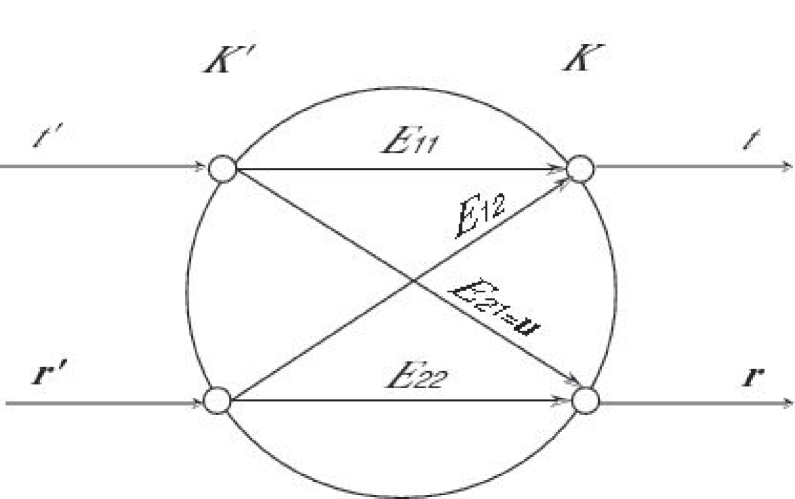
Figure 2: The cascade connection for space-time transformations. The circle represents a black box. One side has two input ports: the time $t^{\prime}$ and the space $\mathbf{r}^{\prime}$ coordinates of an event in system $K^{\prime}$. The other side has two output ports: the time $t$ and the space $\mathbf{r}$ coordinates of the same event in system $K$. The linear operators $E_{ij}$ represent the functional connections between the corresponding ports.

The cascade connection is the one usually used in special relativity.

We represent the linear transformation induced by the cascade connection by a $4\times 4$ matrix $E$, which we decompose into four block matrix components $E_{ij}$, as follows:

$$\left(\begin{array}[]{c}t\\ \mathbf{r}\end{array}\right)=E\left(\begin{array}[]{c}t^{\prime}\\ \mathbf{r}^{\prime}\end{array}\right)=\left(\begin{array}[]{rr}E_{11}&E_{12}\\ E_{21}&E_{22}\end{array}\right)\left(\begin{array}[]{r}t^{\prime}\\ \mathbf{r}^{\prime}\end{array}\right).$$ (1)

To understand the meaning of the blocks, assume that the system $K^{\prime}$ is an airplane. Let $t^{\prime}$ be the time between two events (say crossing two lighthouses) measured by a clock at rest at $\mathbf{r}^{\prime}=0$ on the airplane. The time difference $t$ of the same two events measured by synchronized clocks at the two lighthouses (in system $K$, the earth) will be equal to $t=E_{11}t^{\prime}$. If we denote the distance between the lighthouses by $\mathbf{r}$, then $\mathbf{r}=E_{21}t^{\prime}$, and $E_{21}$ is the so-called proper velocity of the plane. Generally, the proper velocity $\mathbf{u}$ of an object (the airplane) in an inertial system is the ratio of the space displacement $d\mathbf{r}$ in lab system (the earth) divided by the time interval, called the proper time interval $d\tau$, measured by the clock moving with the object (on the plane). Thus,

$$\mathbf{u}=\frac{d\mathbf{r}}{d\tau}.$$ (2)

2.3.2 Hybrid connection

The second type of connection, called the hybrid connection, uses time of one of the systems, say $t$ of $K$, and the space coordinates $\mathbf{r}^{\prime}$ of the second system $K^{\prime}$, as input, and gives $\left(\begin{array}[]{r}t^{\prime}\\ \mathbf{r}\end{array}\right)$ as output (see Figure 3).

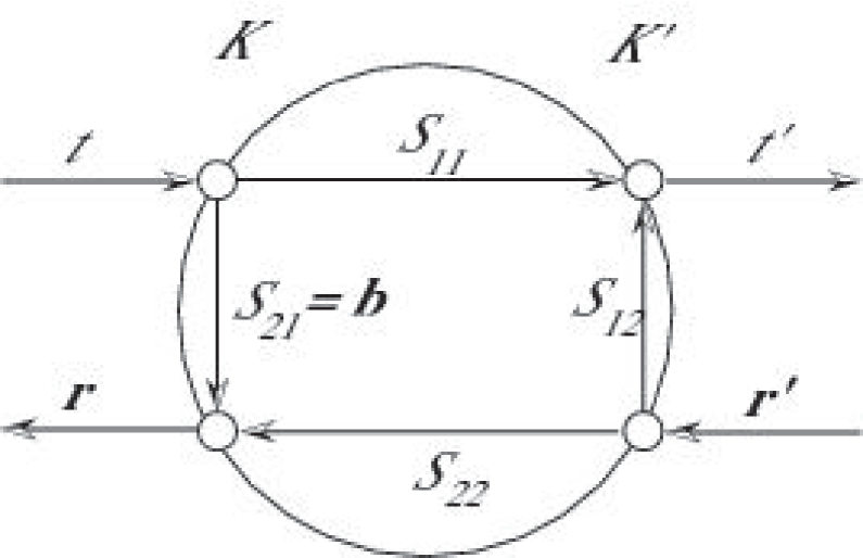
Figure 3: The hybrid connection for space-time transformations. The circle represents a black box. The two input ports are the time $t$ of an event, as measured in system $K$, and its space coordinates $\mathbf{r}^{\prime}$, as measured in system $K^{\prime}$. The two output ports are the time $t^{\prime}$ of the same event, calculated in system $K^{\prime}$, and its space $\mathbf{r}$ coordinates, calculated in $K$. The linear operators $S_{ij}$ represent the functional connections between the corresponding ports. For instance, to define the map $S_{21}$, we consider an event that occurs at $O^{\prime}$, corresponding to input $\mathbf{r}^{\prime}=0$, at time $t$ in $K$. Then $S_{21}t$ represent the space displacement of $O^{\prime}$ in $K$ during time $t$, which is, by the definition, the relative velocity $\mathbf{b}$ of system $K^{\prime}$ with respect to system $K$.

Usually we use relative velocity (not relative proper velocity) to describe the relative position between inertial systems. To define the relative position of system $K^{\prime}$ with respect to $K$, we consider an event that occurs at $O^{\prime}$, corresponding to $\mathbf{r}^{\prime}=0$, at time $t$, and express its position $\mathbf{r}$ in $K$. If we denote by $\mathbf{b}$ the uniform velocity of system $K^{\prime}$ with respect to $K$, then

$$\mathbf{r}=\mathbf{b}t.$$ (3)

Note our use of the hybrid connection. In this section we will use the hybrid connection in order to keep the relative velocity as the description of relative position between the systems. Furthermore, a bounded symmetric domain is obtained only for the velocities and not for the proper velocities.

We denote by $S_{\mathbf{b}}$ the space-time transformation, using the hybrid connection, for two inertial systems with relative velocity $\mathbf{b}$ between them. Thus, for the transformation $S_{\mathbf{b}}$, we choose the inputs to be the scalar $t$, the time of the event in $K$, and the three-dimensional vector $\mathbf{r}^{\prime}$ describing the position of the event in $K^{\prime}$. Then our outputs are the scalar $t^{\prime}$, the time of the event in $K^{\prime}$, and the three-dimensional vector $\mathbf{r}$ describing the position of the event in $K$. As above with respect to the cascade connection, here we also decompose the $4\times 4$ matrix $S_{\mathbf{b}}$ into block components:

$$\left(\begin{array}[]{c}t^{\prime}\\ \mathbf{r}\end{array}\right)=S_{\mathbf{b}}\left(\begin{array}[]{c}t\\ \mathbf{r}^{\prime}\end{array}\right)=\left(\begin{array}[]{rr}S_{11}&S_{12}\\ S_{21}&S_{22}\end{array}\right)\left(\begin{array}[]{r}t\\ \mathbf{r}^{\prime}\end{array}\right).$$ (4)

(see Figure 3).

We explain now the meaning of the four linear maps $S_{ij}$. To define the maps $S_{21}$ and $S_{11}$, consider an event that occurs at $O^{\prime}$, corresponding to $\mathbf{r}^{\prime}=0$, at time $t$ in $K$. Then $S_{21}(t)$ expresses the position of this event in $K$, and $S_{11}(t)$ expresses the time of this event in $K^{\prime}$. Obviously, $S_{21}$ describes the relative velocity of $K^{\prime}$ with respect to $K$, and

$$S_{21}(t)=\mathbf{b}t,$$ (5)

while $S_{11}(t)$ is the time shown by the clock positioned at $O^{\prime}$ of an event occurring at $O^{\prime}$ at time $t$ in $K$ and is given by

$$S_{11}(t)=\alpha t$$ (6)

for some constant $\alpha$.

To define the maps $S_{12}$ and $S_{22}$, we will consider an event occurring at time $t=0$ in $K$ in space position $\mathbf{r}^{\prime}$ in $K^{\prime}$. Then $S_{12}(\mathbf{r}^{\prime})$ will be the time of this event in $K^{\prime}$, and $S_{22}(\mathbf{r}^{\prime})$ will be the position of this event in $K$. Note that $S_{12}(\mathbf{r}^{\prime})$ is also the time difference of two clocks, both positioned at time $t=0$ at $\mathbf{r}^{\prime}$ in $K^{\prime}$, where the first one was synchronized to the clock at the common origin of the two systems within the frame $K^{\prime}$, and the second one was synchronized to the clock at the origin within the frame $K$. Thus $S_{12}$ describes the non-simultaneity in $K^{\prime}$ of simultaneous events in $K$ with respect to their space displacement in $K^{\prime}$, following from the difference in synchronization of clocks in $K$ and $K^{\prime}$. Since $S_{12}$ is a linear map from $R^{3}$ to $R$, it is given by:

$$S_{12}(\mathbf{r}^{\prime})={\mathbf{e}^{T}}\mathbf{r}^{\prime},$$ (7)

for some vector $\mathbf{e}\in R^{3}$, where $\mathbf{e}^{T}$ denotes the transpose of $\mathbf{e}$. Note that ${\mathbf{e}^{T}}\mathbf{r}^{\prime}$ is the dot product of ${\mathbf{e}}$ and $\mathbf{r}^{\prime}$. See Figure 4 for the connection between the time of events in two inertial systems.

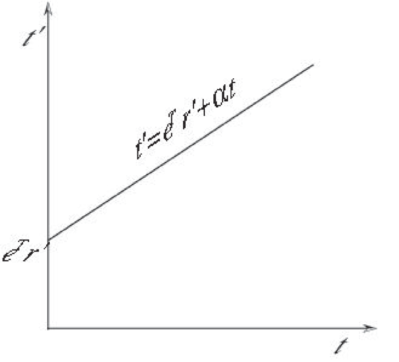
Figure 4: The times $t^{\prime}$ and $t$ of an event at space point $\mathbf{r}^{\prime}$ in system $K^{\prime}$. The difference in timings is caused both by the difference in the rates of clocks (time slowdown) in each system and by the different synchronization of the clocks positioned at different space points.

Finally, the map $S_{22}$ describes the transformation of the space displacement in $K$ of simultaneous events in $K$ with respect to their space displacement in $K^{\prime}$, and it is given by

$$S_{22}(\mathbf{r}^{\prime})=A\mathbf{r}^{\prime}$$ (8)

for some $3\times 3$ matrix $A$.

Note that the usual approach uses the cascade connection for the space-time transformation and the relative velocity, which comes from the hybrid connection, for the description of the relative motion between the systems. However, space contraction, time contraction and the measure of non-simultaneity are defined by use of the hybrid connection.

2.3.3 The transformation between cascade and hybrid connections

Note that the matrices $E$ and $S_{\mathbf{b}}$ describing the space-time transformations between two inertial systems using the cascade and hybrid connections, respectively, are related by some transformation $\Psi$. The transformation is defined by

$$\Psi\left(\begin{array}[]{rr}E_{11}&E_{12}\\ E_{21}&E_{22}\end{array}\right)=\left(\begin{array}[]{cc}E_{11}-E_{12}E_{22}^{-1}E_{21}&E_{12}E_{22}^{-1}\\ -E_{22}^{-1}E_{21}&E_{22}^{-1}\end{array}\right).$$ (9)

This transformation is called the Potapov-Ginzburg transformation. It can be shown that

$$\left(\begin{array}[]{rr}S_{11}&S_{12}\\ S_{21}&S_{22}\end{array}\right)=\Psi\left(\begin{array}[]{rr}E_{11}&E_{12}\\ E_{21}&E_{22}\end{array}\right)$$ (10)

and

$$\left(\begin{array}[]{rr}E_{11}&E_{12}\\ E_{21}&E_{22}\end{array}\right)=\Psi\left(\begin{array}[]{rr}S_{11}&S_{12}\\ S_{21}&S_{22}\end{array}\right).$$ (11)

It is easy to check that $S_{\mathbf{b}}$ is a symmetry (that is, $S_{\mathbf{b}}^{2}=I$) if and only if $E=\Psi(S_{\mathbf{b}})$ is a symmetry.

2.4 Derivation of the explicit form of the symmetry operator

Our black box transformation can now be described by a $4\times 4$ matrix $S_{\mathbf{b}}$ with block matrix entries from (5), (6), (7) and (8):

$$\left(\begin{array}[]{c}t^{\prime}\\ \mathbf{r}\end{array}\right)=S_{\mathbf{b}}\left(\begin{array}[]{c}t\\ \mathbf{r}^{\prime}\end{array}\right)=\left(\begin{array}[]{rr}\alpha&\mathbf{e}^{T}\\ \mathbf{b}&A\end{array}\right)\left(\begin{array}[]{r}t\\ \mathbf{r}^{\prime}\end{array}\right).$$ (12)

If we now interchange the roles of systems $K$ and $K^{\prime}$, we will get a matrix $S^{\prime}_{\mathbf{b}}$:

$$\left(\begin{array}[]{c}t\\ \mathbf{r}^{\prime}\end{array}\right)=S^{\prime}_{\mathbf{b}}\left(\begin{array}[]{c}t^{\prime}\\ \mathbf{r}\end{array}\right)=\left(\begin{array}[]{rr}\alpha^{\prime}&{\mathbf{e^{\prime}}^{T}}\\ \mathbf{b}^{\prime}&A^{\prime}\end{array}\right)\left(\begin{array}[]{r}t^{\prime}\\ \mathbf{r}\end{array}\right).$$ (13)

But the principle of relativity implies that switching the roles of $K$ and $K^{\prime}$ is nonrecognizable. Hence

$$\alpha=\alpha^{\prime},\;\;\mathbf{e}^{T}={\mathbf{e^{\prime}}^{T}},\;\;\mathbf{b}=\mathbf{b}^{\prime},\;\;A=A^{\prime}.$$

By combining (12) and (13), we get $S_{\mathbf{b}}^{2}=I$, implying that $S_{\mathbf{b}}$ is a symmetry operator. Hence,

$$\left(\begin{array}[]{cc}\alpha&\mathbf{e}^{T}\\ \mathbf{b}&A\end{array}\right)\left(\begin{array}[]{rr}\alpha&\mathbf{e}^{T}\\ \mathbf{b}&A\end{array}\right)=\left(\begin{array}[]{rr}1&\mathbf{0}^{T}\\ \mathbf{0}&I\end{array}\right),$$ (14)

where $I$ is the $3\times 3$ identity matrix.

Note that since space is isotropic and the configuration of our systems has one unique divergent direction $\mathbf{b}$, the vector $\mathbf{e}$ is collinear to $\mathbf{b}$. Thus

$$\mathbf{e}=e\mathbf{b}$$ (15)

for some constant $e$. Since the choice of direction of the space coordinate system in the frame is free, the constant $e$ depends only on $|\mathbf{b}|$ and not on $\mathbf{b}$. Finally, from (7) and (15), it follows that this constant has units (length/time)^-2.

Equation (14) implies

$$\alpha=\sqrt{1-e|\mathbf{b}|^{2}}.$$ (16)

and

$$S_{22}=A=-\alpha P_{\mathbf{b}}-(I-P_{\mathbf{b}}),$$ (17)

where $P_{\mathbf{b}}$ denotes the orthogonal projection from space $R^{3}$ onto the direction of $\mathbf{b}$. Thus, the space-time transformation between the two inertial frames $K$ and $K^{\prime}$ is

$$\left(\begin{array}[]{c}t^{\prime}\\ \mathbf{r}\end{array}\right)=S_{\mathbf{b}}\left(\begin{array}[]{c}t\\ \mathbf{r}^{\prime}\end{array}\right)=\left(\begin{array}[]{cc}\alpha&e\mathbf{b}^{T}\\ \mathbf{b}&-\alpha P_{\mathbf{b}}-(I-P_{\mathbf{b}})\end{array}\right)\left(\begin{array}[]{c}t\\ \mathbf{r}^{\prime}\end{array}\right),$$ (18)

with $\alpha$ defined by (16) (see Figure 5).

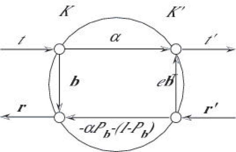
Figure 5: The hybrid connection for space-time transformations between two inertial systems with symmetric frames. The circle represents a black box. The two input ports are the time $t$ of an event, as measured in system $K$, and its space coordinates $\mathbf{r}^{\prime}$, as measured in system $K^{\prime}$. The two output ports are the time $t^{\prime}$ of the same event, calculated in system $K^{\prime}$, and its space $\mathbf{r}$ coordinates, calculated in $K$. The explicit form of the linear operators representing the functional connections between the corresponding ports is shown.

To compare this result with the usual space-time transformations in special relativity, we have to recalculate our result for the cascade connection and reverse the space axes to make them parallel, as usual. To obtain $\left(\begin{array}[]{c}t\\ \mathbf{r}\end{array}\right)$ as a function of $\left(\begin{array}[]{c}t^{\prime}\\ \mathbf{r}^{\prime}\end{array}\right)$ , we use the map $\Psi$ from (11) and obtain

$$\left(\begin{array}[]{c}t\\ \mathbf{r}\end{array}\right)=\Psi(S_{\mathbf{b}})\left(\begin{array}[]{c}t^{\prime}\\ \mathbf{r}^{\prime}\end{array}\right)=\gamma\left(\begin{array}[]{cc}1&e\mathbf{b}^{T}\\ \mathbf{b}&P_{\mathbf{b}}+\gamma^{-1}(I-P_{\mathbf{b}})\end{array}\right)\left(\begin{array}[]{c}t^{\prime}\\ \mathbf{r}^{\prime}\end{array}\right),$$ (19)

where

$$\gamma=\gamma(\mathbf{b})=1/\sqrt{1-e|\mathbf{b}|^{2}}.$$ (20)

This defines an explicit form for the operators of the space-time transformations using the cascade connection (see Figure 6). If $e=0$, then $\gamma=1$, and the transformations are the Galilean transformations.

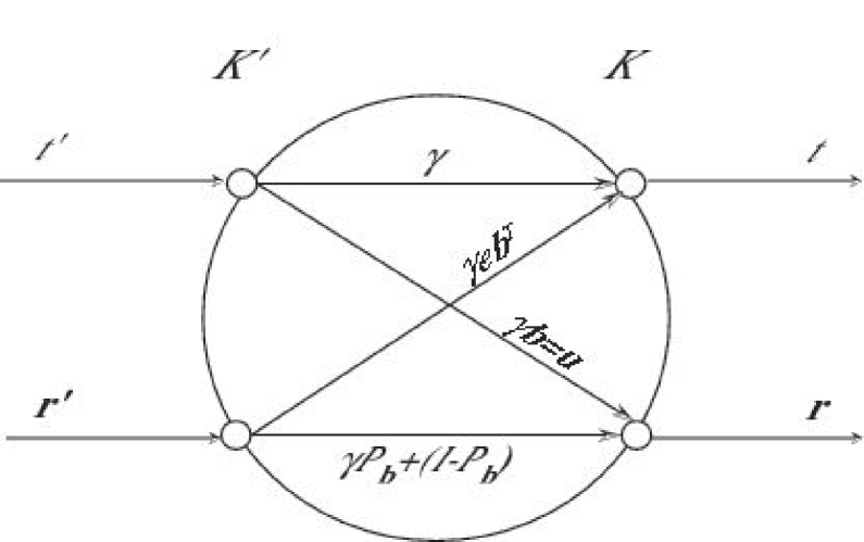
Figure 6: The cascade connection for space-time transformations between two inertial systems $K$ and $K^{\prime}$, moving parallel to $K$ with relative velocity $\mathbf{b}$. The two input ports are the time $t^{\prime}$ of an event and its space coordinates $\mathbf{r}^{\prime}$ , as measured in system $K^{\prime}$, and the two output ports are the time $t$ of the same event and its space $\mathbf{r}$ coordinates, calculated in lab frame $K$. The explicit form of the linear operators representing the functional connections between the corresponding ports is shown.

For the particular case $\mathbf{b}=(v,0,0)$, we get

$$\begin{array}[]{cl}t&=\gamma(t^{\prime}+evx^{\prime})\\ x&=\gamma(vt^{\prime}+x^{\prime})\\ y&=y^{\prime}\\ z&=z^{\prime}\end{array}$$ (21)

which are the usual Lorentz transformations provided $e=1/c^{2}$, which will be shown in the next section.

3 Identification of invariants

In this section we will show that if the transformations are not Galilean, the principle of relativity alone implies that an interval is conserved and that all velocities are limited by some universal velocity. To show this, we introduce an appropriate metric on the space-time under which the symmetry $S_{\mathbf{b}}$ becomes an isometry and a self-adjoint operator. It is known that $S_{\mathbf{b}}$ is self-adjoint with respect to some inner product if and only if the eigenvectors of this operator which correspond to different eigenvalues are orthogonal to each other.

Any symmetry is a reflection with respect to the set of fixed points. Direct verification shows that the events fixed by the transformation $S_{\mathbf{b}}$ lie on a straight world-line through the origin of both frames at time $t=0$, moving with velocity $\mathbf{w}_{1}$ (the 1 eigenvector of $S_{\mathbf{b}}$) defined by

$$\mathbf{w}_{1}:=\frac{\mathbf{b}}{\alpha+1},$$ (22)

where $\alpha$ is defined by (16). The velocity $\mathbf{w}_{1}$ is called the symmetric velocity between the systems $K$ and $K^{\prime}$. The symmetric velocity has the following physical interpretation. Place two objects of equal mass (test masses) at the origins of each inertial system. The center of mass of the two objects will be called the center of the two inertial systems. The symmetric velocity is the velocity of each system with respect to the center of the systems.

Similarly, one finds the -1 eigenvectors of $S_{\mathbf{b}}$, which is defined by

$$\mathbf{w}_{-1}:=\frac{\mathbf{b}}{\alpha-1}.$$ (23)

The new inner product is obtained by leaving the inner product of the space components unchanged and introducing an appropriate weight $\mu$ for the time component. The orthogonality of the eigenvectors means that

$$\langle\left(\begin{array}[]{c}\mu t\\ \mathbf{w}_{1}t\end{array}\right)|\left(\begin{array}[]{c}\mu t\\ \mathbf{w}_{-1}t\end{array}\right)\rangle=t^{2}(\mu^{2}+\langle\mathbf{w}_{1}|\mathbf{w}_{-1}\rangle)=0.$$ (24)

By use of (22), (23) and (16), this becomes

$$\mu^{2}+\frac{|\mathbf{b}|^{2}}{(\alpha+1)(\alpha-1)}=\mu^{2}+\frac{|\mathbf{b}|^{2}}{\alpha^{2}-1}=\mu^{2}-\frac{1}{e}=0.$$ (25)

The orthogonality of the 1 and -1 eigenvectors of $S_{\mathbf{b}}$ is achieved, if $e>0$, by setting

$$\mu=\frac{1}{\sqrt{e}}.$$ (26)

In this case, $S_{\mathbf{b}}$ becomes an isometry with respect to the inner product with weight $\mu$, implying that

$$(\mu t)^{2}+|\mathbf{r}^{\prime}|^{2}=(\mu t^{\prime})^{2}+|\mathbf{r}|^{2},$$ (27)

or, equivalently,

$$(\mu t^{\prime})^{2}-|\mathbf{r}^{\prime}|^{2}=(\mu t)^{2}-|\mathbf{r}|^{2}.$$ (28)

The previous equation implies that our space-time transformation from $K$ to $K^{\prime}$ conserves the relativistic interval

$$ds^{2}=(\mu dt)^{2}-|d\mathbf{r}|^{2},$$ (29)

with $\mu$ defined by (26) and determined be the process of synchronization of the clocks.

In particular, the transformation $S_{\mathbf{b}}$ maps zero interval world-lines to zero interval world-lines. Since zero interval world-lines correspond to uniform motion with unique speed $\mu$, for any relativistic space-time transformation between two inertial systems with $e>0$, there is a speed $\mu$ defined by (26) which is conserved. Obviously, the cone $ds^{2}>0$, corresponding to the positive Lorentz cone, is also preserved under this transformation.

It can be shown that $e$ is independent of the relative velocity $\mathbf{b}$ between the frames $K$ and $K^{\prime}$.

Several experiments at end of 19th century showed that the speed of light is the same in all inertial systems. Thus

$$\mu=c\;\;\mbox{ and }\;\;e=\frac{1}{c^{2}},$$ (30)

where $c$ is the speed of light in a vacuum. Based on this, we can rewrite (16) and (20) as

$$\alpha(\mathbf{b})=\sqrt{1-\frac{|\mathbf{b}|^{2}}{c^{2}}},\;\gamma(\mathbf{b})=\frac{1}{\sqrt{1-\frac{|\mathbf{b}|^{2}}{c^{2}}}}$$ (31)

and the space-time transformations (19) and (21) between two inertial systems are the Lorentz transformations.

If $e=0$, the above space-time transformations become the Galilean transformations and in this case no velocity is preserved. It can be shown that the case $e<0$ leads to physically absurd results, leaving only two possibilities for relativistic space-time transformations: the Galilean and Lorentz transformations.

Since in the Minkowski metric $\mathbf{w}_{1}$ is orthogonal to $\mathbf{w}_{-1}$, the matrix $S_{\mathbf{b}}$ is self-adjoint. Therefore, the adjoint of the relative velocity $\mathbf{b}$, as a linear operator from time to space, is the operator of non-simultaneity of a system $K^{\prime}$ moving with relative velocity $\mathbf{b}$ with respect to the lab frame.

4 Velocity addition and symmetry of the velocity ball

Relativistic velocity addition can be derived from the Lorentz space-time transformation (19) between two inertial systems as follows. Consider two inertial systems $K$ and $K^{\prime}$, moving with relative velocity (boost) $\mathbf{b}$ and a motion with uniform velocity $\mathbf{v}$ in system $K^{\prime}$. The world line of this motion is $\left(\begin{array}[]{c}t^{\prime}\\ \mathbf{v}t^{\prime}\end{array}\right)$ in $K^{\prime}$. From (19) and by use of (30) this world line in system $K$ is

$$\gamma\left(\begin{array}[]{c}t^{\prime}+\frac{\mathbf{b}^{T}\mathbf{v}t^{\prime}}{c^{2}}\\ \mathbf{b}t^{\prime}+t^{\prime}P_{\mathbf{b}}\mathbf{v}+\alpha t^{\prime}(I-P_{\mathbf{b}})\mathbf{v}\end{array}\right)$$

or

$$\gamma t^{\prime}\left(\begin{array}[]{c}1+\frac{\langle\mathbf{b}|\mathbf{v}\rangle}{c^{2}}\\ \mathbf{b}+\mathbf{v}_{\|}+\alpha\mathbf{v}_{\bot}\end{array}\right),$$ (32)

where $\mathbf{v}_{\|}=P_{\mathbf{b}}\mathbf{v}$ denotes the component of $\mathbf{v}$ parallel to $\mathbf{b}$ and $\mathbf{v}_{\bot}=(I-P_{\mathbf{b}})\mathbf{v}$ denotes the component of $\mathbf{v}$ perpendicular to $\mathbf{b}.$ The world line in system $K$ is a straight line corresponding to the velocity, called the relativistic velocity sum $\mathbf{b}\oplus\mathbf{v}.$ This velocity is obtained by dividing the space by the time on the line and is

$$\mathbf{b}\oplus\mathbf{v}=\frac{\mathbf{b}+\mathbf{v}_{\|}+\alpha\mathbf{v}_{\bot}}{1+\frac{\langle\mathbf{b}|\mathbf{v}\rangle}{c^{2}}},$$ (33)

with $\alpha=\alpha(\mathbf{b})=\sqrt{1-|\mathbf{b}|^{2}/c^{2}}$. This is the well-known Einstein velocity addition formula.

In case $\mathbf{b}$ and $\mathbf{v}$ are parallel, this formula becomes:

$$\mathbf{b}\oplus\mathbf{v}=\frac{\mathbf{b}+\mathbf{v}}{1+\frac{{b}{v}}{c^{2}}},$$ (34)

and in case $\mathbf{v}$ is perpendicular to $\mathbf{b}$ the formula becomes:

$$\mathbf{b}\oplus\mathbf{v}=\mathbf{b}+\alpha(\mathbf{b})\mathbf{v}.$$ (35)

Note that the velocity addition is commutative only for parallel velocities.

We denote by $D_{v}$ the set of all relativistically admissible velocities in an inertial frame $K$. This set is defined by

$$D_{v}=\{\mathbf{v}:\;\mathbf{b}\in R^{3},\;|\mathbf{b}|<c\}.$$ (36)

The Lorentz transformation (19) acts on the velocity ball $D_{v}$ as

$$\varphi_{\mathbf{b}}(\mathbf{v})=\mathbf{b}\oplus\mathbf{v}=\frac{\mathbf{b}+\mathbf{v}_{\|}+\alpha\mathbf{v}_{\bot}}{1+\frac{\langle\mathbf{b}|\mathbf{v}\rangle}{c^{2}}}.$$ (37)

It can be shown [7] that the map $\varphi_{\mathbf{b}}$ is a projective (preserving line segments) map of $D_{v}$. We denote by $Aut_{p}(D_{v})$ the group of all projective automorphisms of the domain $D_{v}$. The map $\varphi_{\mathbf{b}}$ belongs to $Aut_{p}(D_{v}).$ It transforms any relativistically admissible velocity $\mathbf{v}\in D_{v}$ of the system $K^{\prime}$, which is moving parallel to $K$ with relative velocity $\mathbf{b}$, to a corresponding unique velocity $\varphi_{\mathbf{b}}(\mathbf{v})\in D_{v}$ in $K$. The existence of such a map shows that the ball $D_{v}$ is homogeneous in the sense that any two points of this ball can be exchanged by an element of $Aut_{p}(D_{v}).$ Moreover, the ball $D_{v}$ is a bounded symmetric domain, meaning that for any point in $D_{v}$ there exist a symmetry belonging to $Aut_{p}(D_{v})$ which fixes only this point.

By a simple argument one can show that the group $Aut_{p}(D_{v})$ of all projective automorphisms is

$$Aut_{p}(D_{v})=\{\varphi_{\mathbf{b},U}=\varphi_{\mathbf{b}}U:\mathbf{b}\in D_{v},\;U\in O(3)\},$$ (38)

where $O(3)$ denotes the orthogonal matrix of size $3\times 3$. This group represents the velocity transformation between two arbitrary (even non-parallel) inertial systems and provides a representation of the Lorentz group.

Note that the Lorentz group representation defined by space-time transformations (19) between two inertial systems is valid only if the systems move in parallel and at time $t=0$ the origins of the two systems coincide, while the velocity transformation (38) between two inertial systems holds for arbitrary systems without any limitation.

5 Kinematics of relativistically accelerated systems

The ideas used for inertial systems can also be applied with some modifications to uniformly accelerated systems. To understand why we are justified in applying our method used for the inertial systems to accelerated systems and what modifications are needed, consider the table in Figure 7, which clarifies our line of reasoning.

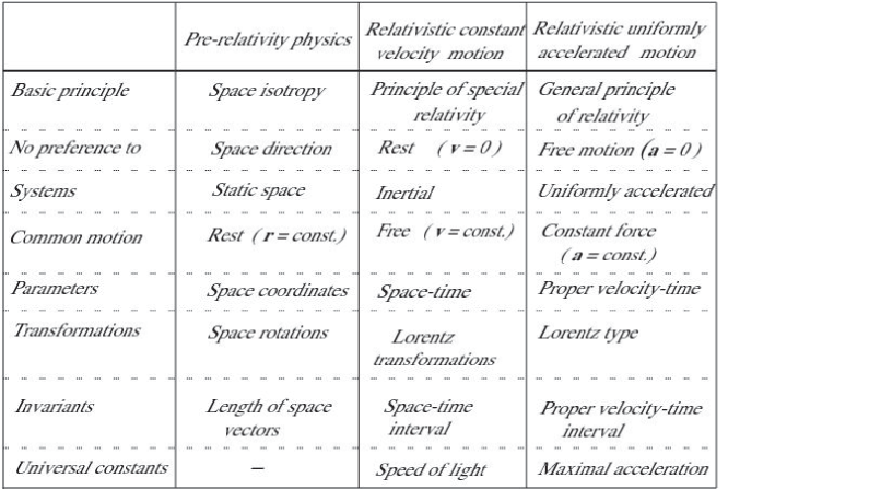
Figure 7: Comparisons between inertial and uniformly accelerated systems.

It highlights three areas of physics:

• Pre-relativity physics, which deals with static space

• Relativistic physics, which deals with arbitrary inertial systems

• Relativistic physics, which deals with systems that are accelerated with respect to inertial systems.

Each of these three areas mentioned has its basic principle which states that the laws of physics are independent of a particular choice. In pre-relativity physics, the laws are independent of the choice of a preferred space direction. In special relativity, the laws are independent of the choice of a preferred inertial system. In general relativity, they are independent of the choice of an arbitrary system.

Pre-relativity physics abandons the notion of a preferred space direction but maintains a preference for rest $(\mathbf{v}=0)$. Special relativity, describing uniform motion, abandons the preference for rest but maintains a preference for constant velocity $(\mathbf{a}=0)$. Here the preferred type of motion is free motion - a motion which is free in one inertial system is free in every inertial system. For accelerated motion, the Principle of General relativity abandons the preference for constant velocity. Even though there is absolutely no preference for any particular kind of accelerated system, we will give preference to uniformly accelerated systems, meaning systems that are uniformly accelerated with respect to an inertial system. The preferred type of motion will thus be motion under a constant force.

For relativistic constant velocity motion, we use the space-time description of events because it is the simplest one which leads to linear transformations between inertial systems. However, it is impossible to obtain linear transformations between uniformly accelerated systems using the space-time description. Consequently, for accelerated comoving systems, we will use a new description, called the proper velocity-time description. This will enable us to obtain linear transformations between comoving uniformly accelerated systems.

Each of these three areas of physics has its own invariants. For constant velocity motion, our method [7] produced transformations which preserve a space-time interval and a maximal speed $c$- the speed of light. Similarly, for uniformly accelerated motion, our method will produce transformations which preserve a proper velocity-time interval and a maximal acceleration.

5.1 Proper acceleration

From (2), (6) and (31) the proper velocity of an object $\mathbf{u}$ is

$$\mathbf{u}=\frac{d\mathbf{r}}{d\tau}=\gamma(\mathbf{v})\mathbf{v}=\frac{\mathbf{v}}{\sqrt{1-{|\mathbf{v}|^{2}}/{c^{2}}}},$$ (39)

where $d\tau=\sqrt{1-{|\mathbf{v}|^{2}}/{c^{2}}}dt$ is the proper time interval, i.e., the time interval in the frame moving with the object. For brevity, we will call proper velocity p-velocity. Note that a p-velocity is expressed as a vector of $R^{3}$. Conversely, any vector in $R^{3}$, with no limitation on its magnitude, represents a relativistically admissible p-velocity.

The principle of equivalence states that “the laws of physics have the same form in a uniformly accelerated system as they do in an unaccelerated inertial system in a uniform gravitational field.” But what is the meaning of uniform acceleration in this principle? Consider an inertial system in a constant gravitational field $G$. If we position an object freely in this system, then, from the relativistic dynamic equation, which we write as

$$m_{0}\frac{d\mathbf{u}}{dt}=G,$$ (40)

we obtain that $\frac{d\mathbf{u}}{dt}$ remains constant. We define proper acceleration $\mathbf{g}$ to be the derivative of p-velocity with respect to time $t$, i.e.,

$$\mathbf{g}=\frac{d\mathbf{u}}{dt}=\frac{d^{2}\mathbf{r}}{dtd\tau}.$$ (41)

This definition coincides with the one given in [11] p.71. By this definition, a free object in an inertial system with a constant gravitational field has constant proper acceleration. By the Equivalence Principle a uniformly accelerated system has to be one in which the origin moves with constant proper acceleration. The magnitude of the proper acceleration is larger then the usual acceleration $\frac{d^{2}\mathbf{r}}{dt^{2}}$, but for small velocities, the magnitudes are almost the same.

By uniformly accelerated system in this paper we will mean systems that are moving with constant proper acceleration with respect to a given inertial system. As mentioned earlier, we will describe first the transformation between an inertial system and uniformly accelerated system (in sense of constant proper acceleration).

5.2 Proper velocity - time description of events

An important step in our derivation of the Lorentz space-time transformations between two inertial frames was to show that such transformations are linear. For uniformly accelerated systems, the space-time transformation is not linear. But, there is another description of events, called the proper velocity - time description, in which the transformation of events between two uniformly accelerated systems is linear.

In the p-velocity-time description, an event is described by the time at which the event occurred and the p-velocity $\mathbf{u}\in R^{3}$ of the event. Thus, an event in the p-velocity-time description is described by a vector $\left(\begin{array}[]{c}t\\ \mathbf{u}\end{array}\right)$ in $R^{4}$. The evolution of an object is described by the p-velocity $\mathbf{u}(t)$ of the object at time $t$, replacing the world-line of special relativity. To obtain the position of the object at time $t$, we have to know the initial position of the object and then integrate its velocity, expressed uniquely by the p-velocity, with respect to time.

For example, for a free-falling object which at time $t=0$ was at rest and positioned at the space frame origin, the p-velocity of this object at time $t$ is $\mathbf{u}(t)=\mathbf{g}t$, where $\mathbf{g}$ is the proper acceleration generated by the gravitational field.

By the principle of equivalence and (40), the motion of an object under the influence of a constant force in a uniformly accelerated system is equivalent to its motion in a constant gravitational field. This motion is described by a straight line in the p-velocity-time continuum. Conversely, if the motion of an object in the p-velocity-time continuum of a uniformly accelerated system is described by a straight line, then the object is under the influence of a constant force.

Two systems moving parallel to each other are called comoving if at some initial time $t_{0}$ their relative velocity is zero. Consider now two comoving systems $K_{g}$ and $K_{0}$, uniformly accelerated with respect to an inertial system $K$ with a constant acceleration $\mathbf{g}$ between them. We assume that at time $t=0$ the relative velocity of $K_{0}$ with respect to $K_{g}$ is zero.

Denote by $T$ the transformation mapping the time and p-velocity $\left(\begin{array}[]{c}t\\ \mathbf{u}\end{array}\right)$ of an event, measured in $K_{g}$, to the time and p-velocity of the same event $\left(\begin{array}[]{c}t^{\prime}\\ \mathbf{u}^{\prime}\end{array}\right)$, measured in $K_{0}$. As we have stated, motion under a constant force in one uniformly accelerated system with respect to an inertial system $K$ is equivalent to motion under a different, but constant, force in $K$. Thus, motion under a constant force in one accelerated system with respect to an inertial system $K$ will be of the same type in any other system uniformly accelerated with respect to $K$. Since such motion is described by a straight line in p-velocity time continuum, this implies that the map $T$ preserves straight lines. We also assumed that relative velocity of $K_{0}$ with respect to $K_{g}$ is zero at time $t=0$. Thus, by a known theorem in mathematics, maps preserving straight lines and mapping the origin to the origin are linear. Since $T$ satisfies these conditions, the transformation $T$ is a linear map.

5.3 Identification of symmetry

To define the symmetry operator between two uniformly accelerated systems, we will use an extension of the principle of relativity, which we will call the General Principle of Relativity. This principle, as it was formulated by M. Born (see [2], p. 312), states that the “laws of physics involve only relative positions and motions of bodies. From this it follows that no system of reference may be favored a priori as the inertial systems were favored in special relativity.”

The principle of relativity from special relativity states that there is no preferred inertial system, and, therefore, the notion of rest (zero velocity) is a relative notion. The motions which were common for all inertial systems are the free (constant velocity) motions. From the general principle of relativity, it follows that there is no preference for inertial (zero acceleration) systems. Hence, when considering accelerated systems, we no longer give preference to free motion (zero force) over constant force motion. This makes all uniformly accelerated systems equivalent. The motion which is common for all accelerated systems is motion under a constant force.

From the general principle of relativity, it is logical to assume that the transformations between the descriptions of an event in two uniformly accelerated systems depend only on the relative motion between these systems. Thus, if we choose reference frames in the two uniformly accelerated systems $K_{g}$ and $K_{0}$ in a way that the description of relative motion of $K_{0}$ with respect to $K_{g}$ coincides with the description of relative motion of $K_{g}$ with respect to $K_{0}$, then the transformation $T$, defined above, will coincide with the transformation $\widetilde{T}$ from $K_{0}$ to $K_{g}$. This implies that $T$ is a symmetry.

In order for this transformation to be a symmetry, we have to choose the space axes in such a way that the description of the relative position of system two with respect to system one coincides with the description of the relative position of system one with respect to system two. This can be done in the same way as was done for inertial systems in Section 2.2. By reversing the p-velocity axes in $K_{0}$ we can make the relative acceleration of $K_{g}$ with respect to $K_{0}$ also be $\mathbf{g}$.

In order to describe the precise meaning of “the system $K_{0}$ moves with uniform acceleration $\mathbf{g}$ with respect to $K_{g}$,” we consider an event connected to an object which is at rest at $O^{\prime}$-the origin of $K_{0}$. The p-velocity of this object in $K_{0}$ is $\mathbf{u}^{\prime}=0$. The acceleration of system $K_{0}$ with respect to $K_{g}$ expresses the p-velocity $\mathbf{u}$ of this object after time $t$ in $K_{g}$. Thus, p-velocity in system $K_{0}$ and time in $K_{g}$ served as inputs and p-velocity in $K_{g}$ as an output. This corresponds to the hybrid connection discussed in Section 2.3.2.

The p-velocity-time transformation $S_{\mathbf{g}}$ between these frames can be considered as a “two-port linear black box” transformation with two inputs and two outputs. In each system, the time and the p-velocity of an event are the two ports. We choose the inputs to be the scalar $t$, the time of the event in $K_{g}$, and the three-dimensional vector $\mathbf{u}^{\prime}$ describing the p-velocity of the event in $K_{0}$. Then the outputs are the scalar $t^{\prime}$, the time of the event in $K_{0}$, and the three-dimensional vector $\mathbf{u}$ describing the p-velocity of the event in $K_{g}$. We denote by $S_{\mathbf{g}}$ mapping $\left(\begin{array}[]{c}t\\ \mathbf{u}^{\prime}\end{array}\right)$ to $\left(\begin{array}[]{c}t^{\prime}\\ \mathbf{u}\end{array}\right),$ which is uniquely defined by $T$. The symmetry of the p-velocity-time transformation $T$ implies (see [7]) that also the transformation $S_{\mathbf{g}}$ is a symmetry and the linearity of $T$ implies the linearity of the transformation $S_{\mathbf{g}}$.

5.4 Identification of the transformation

The map $S_{\mathbf{g}}$ can be represented by a $4\times 4$ matrix. The four block components of the transformation $S_{\mathbf{g}}$, defined by

$$\left(\begin{array}[]{c}t^{\prime}\\ \mathbf{u}\end{array}\right)=S_{\mathbf{g}}\left(\begin{array}[]{c}t\\ \mathbf{u}^{\prime}\end{array}\right)=\left(\begin{array}[]{rr}S_{11}&S_{12}\\ S_{21}&S_{22}\end{array}\right)\left(\begin{array}[]{r}t\\ \mathbf{u}^{\prime}\end{array}\right),$$ (42)

will be denoted by $S_{ij}$, for $i,j\in\{1,2\}$, as in Figure 3.

Obviously, $S_{21}=\mathbf{g}$. The map $S_{11}$ describes the transformation of the time $t$ in $K_{g}$ of an event with p-velocity $\mathbf{u}^{\prime}=0$ (at rest in $K_{0}$) to its time $t^{\prime}$ in $K_{0}$, and it is given by

$$t^{\prime}=S_{11}(t)=\beta t,$$ (43)

for some constant $\beta$. The constant $\beta$ expresses the slowdown of the clocks at rest in $K_{0}$ due to its acceleration relative to $K_{g}$. The value of $\beta$ is related to the well-known Clock Hypothesis. Recall that the Clock Hypothesis states that the “rate of an accelerated clock is identical to that of instantaneously comoving inertial clock.” Now the p-velocity of $K_{0}$ with respect to $K_{g}$ was zero at time $t=0$. Therefore, at time $t=0$, both $K_{0}$ and $K_{g}$ have the same comoving inertial system. Thus, the clock hypothesis would imply $\beta=1$.

To define the maps $S_{12}$ and $S_{22}$, we will consider an event occurring at time $t=0$ in $K_{g}$ with p-velocity $\mathbf{u}^{\prime}$ measured in $K_{0}$. Then $S_{12}(\mathbf{u}^{\prime})$ will be the time of this event in $K_{0}$, and $S_{22}(\mathbf{u}^{\prime})$ will be the p-velocity of this event in $K_{g}$. Since $S_{12}$ is a linear map from $R^{3}$ to $R$, we have

$$S_{12}(\mathbf{u}^{\prime})=<\mathbf{h}|\mathbf{u}^{\prime}>={\mathbf{h}^{T}}\cdot\mathbf{u}^{\prime},$$ (44)

for some vector $\mathbf{h}\in R^{3}$. $S_{12}(\mathbf{u}^{\prime})$ measures the non-synchronization in $K_{0}$ at $t=0$ of two clocks, one at rest and one moving with constant p-velocity $\mathbf{u}^{\prime}$ in $K_{0}$, where both clocks were synchronized at $t=0$ in system $K_{g}$.

Note that since space is isotropic and the configuration of our systems has one unique divergent direction $\mathbf{g}$, the vector $\mathbf{h}$ is collinear to $\mathbf{g}$. Thus

$$\mathbf{h}=\kappa\mathbf{g},$$ (45)

for some constant $\kappa$. Since the choice of direction of the space coordinate system in the frame is free, the constant $\kappa$ depends only on $|\mathbf{g}|$ and not on $\mathbf{g}$. From (44) and (45), it follows that this constant has units $(length/time^{2})^{-2}$.

The map $S_{22}$ describes the p-velocity difference in $K_{g}$ of simultaneous events in $K_{g}$ with respect to their p-velocity difference in $K_{0}$, and it is given by

$$S_{22}(\mathbf{u}^{\prime})=A\mathbf{u}^{\prime}$$ (46)

for some $3\times 3$ matrix $A$.

Our black box transformation can now be described by a $4\times 4$ matrix $S_{\mathbf{g}}$ with block matrix entries from (43), (44), (45) and (46), as

$$S_{\mathbf{g}}=\left(\begin{array}[]{rr}\beta&\kappa\mathbf{g}^{T}\\ \mathbf{g}&A\end{array}\right).$$ (47)

Since $S_{\mathbf{g}}$ is a symmetry operator, it follows that $S_{\mathbf{g}}^{2}=I$-the identity. Hence,

$$\left(\begin{array}[]{cc}\beta&\kappa\mathbf{g}^{T}\\ \mathbf{g}&A\end{array}\right)\left(\begin{array}[]{rr}\beta&\kappa\mathbf{g}^{T}\\ \mathbf{g}&A\end{array}\right)=\left(\begin{array}[]{rr}1&\mathbf{0}^{T}\\ \mathbf{0}&I\end{array}\right),$$ (48)

where $I$ is the $3\times 3$ identity matrix.

From the multiplication of the first row by the first column we have $\beta^{2}+\kappa|\mathbf{g}|^{2}=1$ and, thus

$$\beta=\sqrt{1-\kappa|\mathbf{g}|^{2}}.$$ (49)

From the multiplication of the last 3 rows row by the last 3 columns we have $\kappa\mathbf{g}\mathbf{g}^{T}+A^{2}=I.$ Using that $\mathbf{g}\mathbf{g}^{T}=|\mathbf{g}|^{2}P_{\mathbf{g}},$ where $P_{\mathbf{g}}$ denotes the orthogonal projection on the direction of $\mathbf{g},$ we get $A^{2}=I-\kappa|\mathbf{g}|^{2}P_{\mathbf{g}}=\beta^{2}P_{\mathbf{g}}-(I-P_{\mathbf{g}}).$ Thus,

$$A=-\beta P_{\mathbf{g}}-(I-P_{\mathbf{g}}).$$ (50)

The negative sign is chosen because of the space reversal of axes. Thus, the p-velocity-time transformation between the two frames $K_{g}$ and $K_{0}$ is

$$\left(\begin{array}[]{c}t^{\prime}\\ \mathbf{u}\end{array}\right)=S_{\mathbf{g}}\left(\begin{array}[]{c}t\\ \mathbf{u}^{\prime}\end{array}\right)=\left(\begin{array}[]{cc}\beta&\kappa\mathbf{g}^{T}\\ \mathbf{g}&-\beta P_{\mathbf{g}}-(I-P_{\mathbf{g}})\end{array}\right)\left(\begin{array}[]{c}t\\ \mathbf{u}^{\prime}\end{array}\right),$$ (51)

with $\beta$ defined by (49).

Next, to define an explicit form for the operators of the p-velocity-time transformations between two comoving uniformly accelerated systems using the cascade connection, we use the map $\Psi$ from (11) and revers the space axes to make them parallel, as usual. We obtain

$$\left(\begin{array}[]{c}t\\ \mathbf{u}\end{array}\right)=\beta^{-1}\left(\begin{array}[]{cc}1&\kappa\mathbf{g}^{T}\\ \mathbf{g}&P_{\mathbf{g}}+\beta(I-P_{\mathbf{g}})\end{array}\right)\left(\begin{array}[]{c}t^{\prime}\\ \mathbf{u}^{\prime}\end{array}\right).$$ (52)

To compare these transformations with the well known Lorentz transformations, we choose the $x$-axis of $K_{g}$ in the direction of $\mathbf{g}$. Denote $\mathbf{g}=(g,0,0)$, $\mathbf{u}=(u_{x},u_{y},u_{z})$ and $\mathbf{u}^{\prime}=(u^{\prime}_{x},u^{\prime}_{y},u^{\prime}_{z})$. We get

$$\begin{array}[]{cl}t&=\beta^{-1}(t^{\prime}+\kappa gu^{\prime}_{x})\\ u_{x}&=\beta^{-1}(gt^{\prime}+u^{\prime}_{x})\\ u_{y}&=u^{\prime}_{y}\\ u_{z}&=u^{\prime}_{z},\end{array}$$ (53)

which is a Lorentz-type transformation of the p-velocity.

If $\kappa=0$, which corresponds to the assumption of the Clock Hypothesis, then from (49) we have $\beta=1$ and the p-velocity-time transformations (53) become Galilean.

From now on we will consider only the case $\kappa\neq 0$.

6 Conservation of p-velocity time interval and maximal acceleration

As mentioned above, the p-velocity-time transformation between the systems $K_{g}$ and $K_{0}$ is a symmetry transformation. Such a symmetry is a reflection with respect to the set of points fixed by the symmetry. The events fixed by the transformation $S_{\mathbf{g}}$ are on a straight line through the origin of the p-velocity-time continuum, corresponding to the motion of an object with constant acceleration $\mathbf{w}_{1}$ (see Figure 8) in both frames, where $\mathbf{w}_{1}$ is

$$\frac{\mathbf{g}}{1+\beta}=\frac{\mathbf{u}}{t}:=\mathbf{w}_{1}.$$ (54)

Figure 8: Eigenspaces of the symmetry.

The events, which are the -1 eigenvectors of $S_{\mathbf{g}}$ in the plane generated by $\mathbf{g}$ and the $t$-axis, are on a straight line through the origin of the p-velocity-time continuum, corresponding to the motion of an object with constant acceleration $\mathbf{w}_{-1}$, defined as

$$\frac{\mathbf{u}^{\prime}}{t}=\frac{\mathbf{g}}{\beta-1}=\frac{\mathbf{u}}{t}:=\mathbf{w}_{-1}.$$ (55)

The symmetry $S_{\mathbf{g}}$ becomes an isometry if we introduce an appropriate inner product. Under this inner product, the 1 and -1 eigenvectors of $S_{\mathbf{g}}$ will be orthogonal. The new inner product is obtained by leaving the inner product of the p-velocity components unchanged and introducing an appropriate weight $\nu$ for the time component. The orthogonality of the eigenvectors means that

$$<\left(\begin{array}[]{c}\nu t\\ \mathbf{w}_{1}t\end{array}\right)|\left(\begin{array}[]{c}\nu t\\ \mathbf{w}_{-1}t\end{array}\right)>=t^{2}(\nu^{2}+<\mathbf{w}_{1}|\mathbf{w}_{-1}>)=0.$$ (56)

By use of (54), (55) and (49), this becomes

$$\nu^{2}+\frac{|\mathbf{g}|^{2}}{(1+\beta)(\beta-1)}=\nu^{2}-\frac{1}{\kappa}=0.$$ (57)

If $\kappa>0$, this implies that

$$\nu=\frac{1}{\sqrt{\kappa}}.$$ (58)

The value $\nu$ has units of acceleration. From the fact that $S_{\mathbf{g}}$ is an isometry with respect to the inner product with weight $\nu$, we have

$$(\nu t)^{2}+|\mathbf{u}^{\prime}|^{2}=(\nu t^{\prime})^{2}+|\mathbf{u}|^{2},$$ (59)

or, equivalently,

$$(\nu t^{\prime})^{2}-|\mathbf{u}^{\prime}|^{2}=(\nu t)^{2}-|\mathbf{u}|^{2}.$$ (60)

The previous equation implies that our p-velocity-time transformation from $K_{g}$ to $K_{0}$ conserves the interval

$$d\widetilde{s}^{2}=(\nu dt)^{2}-|d\mathbf{u}|^{2},$$ (61)

with $\nu$ defined by (58) and thus is a Lorentz-type transformations.

Note that the zero-interval world-lines are transformed by these transformations to zero-interval lines. The zero-interval world-lines correspond to motion with uniform acceleration $\nu$ depending only on the magnitude $g$ of the relative accelerations between the systems, which we denote by $\nu_{g}$. Thus, for two systems $K_{g}$ and $K_{0}$ with $\kappa>0$, the acceleration $\nu_{g}$ defined by (58) is conserved.

Considering three accelerated comoving systems: where system two is moving in parallel with acceleration $\mathbf{g}$ with respect to system one and system three is moving in parallel with the same acceleration $\mathbf{g}$ with respect to system two we obtain that $\nu_{2g}=\nu_{g}$. By use of an argument similar to the one in [7], section 1.2.2, it can be shown that the conserved acceleration $\nu_{g}$ is independent of the relative acceleration $\mathbf{g}$ between the frames $K_{g}$ and $K_{0}$ and we will denote it by $a_{M}$. From (58)

$$a_{M}=1/\sqrt{\kappa}.$$ (62)

Since the cone $d\widetilde{s}^{2}>0$ is preserved under the p-velocity-time transformation, an acceleration of magnitude less them $a_{M}$ in one uniformly accelerated system will be also of magnitude less them $a_{M}$ in any other uniformly accelerated system. Thus, all relativistically admissible accelerations, belong to a ball $D_{a}$

$$D_{a}=\{\mathbf{a}\in R^{3}:\;\;|\mathbf{a}|<a_{M}\}.$$ (63)

The case $\kappa<0$ is excluded by an argument, similar to the one used in [7], section 1.3.2.

7 The ball of relativistically admissible accelerations $D_{a}$

If the maximal acceleration exists, the constant $\kappa=1/a_{M}^{2}$ and the p-velocity-time transformations (53) become

$$\begin{array}[]{cl}t&=\beta^{-1}(t^{\prime}+\frac{gu^{\prime}_{x}}{a_{M}^{2}})\\ u_{x}&=\beta^{-1}(gt^{\prime}+u^{\prime}_{x})\\ u_{y}&=u^{\prime}_{y}\\ u_{z}&=u^{\prime}_{z},\end{array}$$ (64)

with $\beta=\sqrt{1-\frac{g^{2}}{a_{M}^{2}}}.$ From this one derives a new acceleration addition formula as follows. Consider an object moving with acceleration $\mathbf{a}=(a,0,0)$ in the direction of the of the $x^{\prime}$ axis in $K_{0}$ with zero p-velocity at $t^{\prime}=0$. Its p-velocity in $K_{0}$ is $u^{\prime}_{x}=at^{\prime},u^{\prime}_{y}=0,u^{\prime}_{z}=0$. Thus, the p-velocity-time description of this object in system $K_{g}$ is $t=\beta^{-1}t^{\prime}(1+\frac{ga}{a_{M}^{2}}),u_{x}=\beta^{-1}t^{\prime}(g+a),u_{y}=0,u_{z}=0$. Such motion of this object in $K_{g}$ represents addition of the acceleration $\mathbf{g}$ of the system $K_{0}$ with respect to $K_{g}$ to the acceleration $\mathbf{a}$ of the object with respect to $K_{0}$. Since,

$$\frac{u_{x}}{t}=\frac{g+a}{1+\frac{ga}{a_{M}^{2}}}\mbox{ and }\;\frac{u_{y}}{t}=\frac{u_{z}}{t}=0,$$

the motion is with constant acceleration. This operation is denoted by $\mathbf{g}\oplus\mathbf{a}$ and coincides with the similar formula of Einstein velocity addition (for parallel velocities) in special relativity.

A general acceleration-addition formula for non-parallel accelerations is

$$\mathbf{g}\oplus\mathbf{a}=\frac{\mathbf{g}+\mathbf{a}_{||}+\beta\mathbf{a}_{\bot}}{1+<\mathbf{a}|\mathbf{g}>/a_{M}^{2}},$$ (65)

with $\beta=\sqrt{1-|\mathbf{g}|^{2}/a_{M}^{2}}$, $\mathbf{a}_{||}=P_{\mathbf{g}}\mathbf{a}$ and $\mathbf{a}_{\bot}=(I-P_{\mathbf{g}})\mathbf{a}$. This map defines a projective symmetry making the ball $D_{a}$ into a bounded symmetric domain with respect to $Aut_{p}(D_{a})$.

The existence of a maximal acceleration follows also from Born’s reciprocity principle, which states [2] that the laws of nature are symmetric with respect to space and momentum. We think that “momentum” should be replaced by “proper velocity” in Born’s reciprocity principle. Such reciprocity could not be achieved with the Galilean transformation for the proper-velocity time continuum. As we have shown, this implies the existence of a maximal acceleration. Caianiello’s model [3] also supports Born’s reciprocity principle.As shown by Schuller [14], the Muon Storage Ring experiment (see [1] and [6]) implies that the constant $\kappa<1.6\cdot 10^{-39}(s^{2}/m)^{2}$ and from the relativistic correction of the Thomas precession $\kappa<10^{-44}(s^{2}/m)^{2}$, which is indeed close to zero. From Caianiello’s model, the estimate of the maximal acceleration in Scarpetta [13] is $\kappa=0.4\cdot 10^{-103}(s^{2}/m)^{2}.$ But the existence and the real value of maximal acceleration could be obtained only from experiment, directly or indirectly.

8 Space-time transformations to a uniformly accelerated system without the Clock Hypothesis

As we have shown, if the Clock Hypothesis is not valid, there exist a unique maximal acceleration. Then from (43) and (49), it follows that

$$\tilde{t}=\sqrt{1-\frac{|\mathbf{g}|^{2}}{a_{M}^{2}}}t.$$ (66)

This equation was called the modified Clock hypothesis by Shuller [14]. It shows that the dependence of the rate of an accelerated clock is due to its acceleration as well as its velocity.

At this point we do not know how to obtain an explicit space-time transformation from an inertial system $K$ to a system $\widetilde{K}$ uniformly accelerated with respect to $K$ without assuming the Clock hypothesis. But we can do this for any given world-line $(t,\mathbf{r}(t))$ in $K$ by the following algorithm:

Algorithm: Step 1. Use Lorentz transformations to obtain a world-line $(t^{\prime},\mathbf{r}^{\prime}(t^{\prime}))$ in $K^{\prime}$ the comoving frame to $\widetilde{K}$.

Step 2. Translate this world line $(t^{\prime},\mathbf{r}^{\prime}(t))$ from space-time representation to a world-line $(t^{\prime},\mathbf{u}^{\prime}(t))$ in the p-velocity-time representation in $K^{\prime}$.

Step 3. Use transformation (52) to obtain world-line $(\tilde{t},\tilde{\mathbf{u}}(t))$ in the p-velocity-time representation in $\tilde{K}.$ Finally,

Step 4. Using the formula

$$\mathbf{r}(t)=\int_{0}^{t}\mathbf{v}({\lambda})d\lambda=\int_{0}^{t}\frac{\mathbf{u}(\lambda)d\lambda}{\sqrt{1+|\mathbf{u}(\lambda)|^{2}/c^{2}}}$$ (67)

obtain a world-line $(\tilde{t},\tilde{\mathbf{r}}(t))$ in the space-time representation in $\tilde{K}$ corresponding to the world-line $(t,\mathbf{r}(t))$ in $K$.

We want to thank Michael Danziger for helpful remarks.

References

- [1] J. Bailey et al., Measurements of the relativistic time dilation for positive and negative muons in circular orbit, Nature 268 (1977) 301–305.
- [2] M. Born, Einstein’s Theory of Relativity ( Dover Publications, New York, 1965).
- [3] E. R. Caianiello, Is there a Maximal Acceleration?, Lettere al Nuovo Cimento 32 (1981) 65–70.
- [4] A. Einstein, Zur Elektrodynamik bewegter Körper, Ann. Phys. 17 (1905), 891.
- [5] A. Einstein, The meaning of relativity, Princeton University Press, Princeton, New Jersey, 1955.
- [6] A. M. Eisele, On the behaviour of an accelerated clock, Helvetica Physica Acta 60 (1987) 1024-1037.
- [7] Y. Friedman, Physical Applications of Homogeneous Balls, Progress in Mathematical Physics 40 (Birkhäuser, Boston, (2004).
- [8] Y. Friedman ,Yu. Gofman , Relativistic spacetime transformation based on symmetry, Found. Phys., 32, (2002) 1717–1736.
- [9] Y. Friedman, Yu. Gofman, Kinematic relations between relativistically accelerated systems in flat space-time based on symmetry, arxiv/gr-qc/0509004.
- [10] Y. Friedman, M. Semon, Relativistic acceleration of charged particles in uniform and mutually perpendicular electric and magnetic fields as viewed in the laboratory frame, Phys. Rev. E 72 (2005), 026603.
- [11] W. Rindler, Relativity: Special, General and Cosmological, Oxford University Press (2004)
- [12] G. Scarpetta, Lett. Nuovo Cimento 41 (1984) 51.
- [13] G. Scarpetta, Lett. Nuovo Cimento 41 (1984) 51.
- [14] F. P. Schuller, Born-Infeld Kinematics, Ann. Phys. 299 (2002) 174.