CORRELATION LENGTH AND NEGATIVE PHASE VELOCITY IN ISOTROPIC DIELECTRIC–MAGNETIC MATERIALS

Tom G. Mackay^a and Akhlesh Lakhtakia^b

^a School of Mathematics
University of Edinburgh
Edinburgh EH9 3JZ, United Kingdom
email: T.Mackay@ed.ac.uk

^b CATMAS — Computational & Theoretical Materials Sciences Group
Department of Engineering Science & Mechanics
212 Earth & Engineering Sciences Building
Pennsylvania State University, University Park, PA 16802–6812
email: akhlesh@psu.edu

ABSTRACT: A composite material comprising randomly distributed spherical particles of two different isotropic dielectric–magnetic materials is homogenized using the second–order strong–property–fluctuation theory in the long–wavelength approximation. Whereas neither of the two constituent materials by itself supports planewave propagation with negative phase velocity (NPV), the homogenized composite material (HCM) can. The propensity of the HCM to support NPV propagation is sensitive to the distributional statistics of the constituent material particles, as characterized by a two–point covariance function and its associated correlation length. The scope for NPV propagation diminishes as the correlation length increases.

Keywords: homogenization, strong–property–fluctuation theory, negative refraction

1. INTRODUCTION

The descriptions of electromagnetic planewave propagation traditionally encountered in standard textbooks generally involve positive phase velocity (PPV) — that is, the phase velocity casts a positive projection onto the time–averaged Poynting vector. On the other hand, there is growing recognition of the importance of negative–phase–velocity (NPV) propagation, wherein the phase velocity casts a negative projection onto the time–averaged Poynting vector [1, 2]. Of the many exotic phenomenons that follow as a consequence of NPV, negative refraction has been the focus of particular attention because of its scientific as well as technological significance [3].

Manifestations of NPV are not readily observed in naturally occurring homogeneous materials. In contrast, artificial metamaterials may be conceptualized — and in some instances physically realized — which support NPV propagation. To date, experimental developments with NPV–supporting homogeneous metamaterials have been limited to wavelengths larger than in the visible regime, with the micromorphology based on elements of complicated shapes [4, 5, 6].

In a recent study, we proposed a simple recipe for a NPV–supporting metamaterial, based on the homogenization of a random assembly of two different types of spherical particles [7]. The two types of constituent particles, type $a$ and type $b$, are each made of an isotropic, homogeneous dielectric–magnetic material, the relative permittivities being denoted by $\epsilon_{a,b}$ and the relative permeabilities by $\mu_{a,b}$. Provided that $\epsilon_{a,b}$ and $\mu_{a,b}$ lie within certain parameter ranges, with the real parts of $\epsilon_{a,b}$ being negative–valued and the real parts of $\mu_{a,b}$ being positive–valued (or vice versa), the bulk constituent materials do not support NPV propagation whereas the corresponding homogenized composite material (HCM) does. The constitutive parameters of the HCM were estimated using the well–established Bruggeman homogenization formalism [8]. The Bruggeman approach has the advantages other recent approaches involving NPV–supporting metamaterials [9, 10] that (i) the constituent particles are not resonant, and (ii) it is not limited to dilute composites.

The sizes of the constituent material particles play a significant role in determining whether or not HCMs support NPV propagation [9, 10]. Using an extended Bruggeman approach [11], we recently reported that increasing the particle size diminishes the scope for NPV propagation in the HCM [12]. The role of the distributional statistics of the constituent material particles in NPV–supporting metamaterials has also been highlighted recently [10] — it is this topic that we explore herein.

The Bruggeman homogenization formalism takes into account the distributional statistics of the constituent material particles only at the lowest order, via the volume fractions of the constituent materials. A different approach is provided by the strong–property–fluctuation theory (SPFT) in which a comprehensive description of the distributional statistics of the constituent material particles may be accommodated. The provenance of the SPFT lies in wave–propagation studies for continuous random mediums [13, 14], but it has more recently gained prominence in the homogenization of particulate composites [15]. Within the SPFT, estimates of the HCM’s constitutive parameters are calculated as successive iterates to the constitutive parameters of a homogenous comparison medium. The iterates are expressed in terms of correlation functions describing the spatial distribution of the constituent material particles. In principle, correlation functions of arbitrarily high order can be incorporated.

The SPFT is commonly implemented at the second–order level of approximation wherein the distribution statistics are stated in terms of a two–point correlation function and its associated correlation length [16]. The correlation length is taken to be large relative to the constituent material particles, but small relative to the electromagnetic wavelengths. The electromagnetic responses of constituent material particles within a region of linear dimensions given by the correlation length are mutually dependent, whereas the electromagnetic responses of constituent material particles separated by distances much greater than the correlation length are assumed to be independent [17].

In the following sections, the second–order SPFT is applied to investigate the role of correlation length in predicting whether or not an isotropic dielectric–magnetic HCM supports NPV propagation.

As regards notational matters, $\mbox{Re}\left\{z\right\}$ denotes the real part and $\mbox{Im}\left\{z\right\}$ the imaginary part of a complex–valued scalar $z$. The free–space wavenumber at angular frequency $\omega$ is written as $k_{\scriptscriptstyle 0}=\omega\sqrt{\epsilon_{\scriptscriptstyle 0}\mu_{\scriptscriptstyle 0}}$, with $\epsilon_{\scriptscriptstyle 0}$ and $\mu_{\scriptscriptstyle 0}$ being the permittivity and permeability of free space, respectively.

2. HOMOGENIZATION

Let us consider the homogenization of two constituent materials described in the previous section. Both constituent materials are composed of electrically small spherical particles, which are randomly mixed together. Since materials $a$ and $b$ are assumed to be passive, the principle of causality — combined with the implicit time–dependence $\exp(-i\omega t)$ — imposes the constraint [18]

$$\left.\begin{array}[]{l}\mbox{Im}\,\left\{\epsilon_{\ell}\right\}>0\\ \mbox{Im}\,\left\{\mu_{\ell}\right\}>0\end{array}\right\},\qquad(\ell=a,b).\,$$ (1)

Let $f_{\ell}\in(0,1)$ ($\ell=a,b$) denote the volume fraction of phase $\ell$, with $f_{a}+f_{b}=1$.

The HCM is an isotropic, homogeneous, dielectric–magnetic material. By application of the SPFT, estimates of its relative permittivity $\epsilon_{\scriptscriptstyle HCM}$ and relative permeability $\mu_{\scriptscriptstyle HCM}$ are provided by the iterative refinement of the corresponding constitutive parameters of a homogeneous comparison medium. Furthermore, it transpires that the relative permittivity and relative permeability of the comparison medium are identical to those yielded by the Bruggeman homogenization formalism [15, 17] — namely, $\epsilon_{\scriptscriptstyle Br}$ and $\mu_{\scriptscriptstyle Br}$ [7].

At the second–order level of approximation, the SPFT estimates emerge as [15, 17]

$$\epsilon_{\scriptscriptstyle HCM} = \epsilon_{\scriptscriptstyle Br}\left\{1+\frac{6k^{2}_{\scriptscriptstyle Br}T\left[f_{a}\left(\displaystyle{\frac{\epsilon_{a}-\epsilon_{\scriptscriptstyle Br}}{\epsilon_{a}+2\epsilon_{\scriptscriptstyle Br}}}\right)^{2}+f_{b}\left(\displaystyle{\frac{\epsilon_{b}-\epsilon_{\scriptscriptstyle Br}}{\epsilon_{b}+2\epsilon_{\scriptscriptstyle Br}}}\right)^{2}\right]}{1-2k^{2}_{\scriptscriptstyle Br}T\left[f_{a}\left(\displaystyle{\frac{\epsilon_{a}-\epsilon_{\scriptscriptstyle Br}}{\epsilon_{a}+2\epsilon_{\scriptscriptstyle Br}}}\right)^{2}+f_{b}\left(\displaystyle{\frac{\epsilon_{b}-\epsilon_{\scriptscriptstyle Br}}{\epsilon_{b}+2\epsilon_{\scriptscriptstyle Br}}}\right)^{2}\right]}\right\},$$ (2)

$$\mu_{\scriptscriptstyle HCM} = \mu_{\scriptscriptstyle Br}\left\{1+\frac{6k^{2}_{\scriptscriptstyle Br}T\left[f_{a}\left(\displaystyle{\frac{\mu_{a}-\mu_{\scriptscriptstyle Br}}{\mu_{a}+2\mu_{\scriptscriptstyle Br}}}\right)^{2}+f_{b}\left(\displaystyle{\frac{\mu_{b}-\mu_{\scriptscriptstyle Br}}{\mu_{b}+2\mu_{\scriptscriptstyle Br}}}\right)^{2}\right]}{1-2k^{2}_{\scriptscriptstyle Br}T\left[f_{a}\left(\displaystyle{\frac{\mu_{a}-\mu_{\scriptscriptstyle Br}}{\mu_{a}+2\mu_{\scriptscriptstyle Br}}}\right)^{2}+f_{b}\left(\displaystyle{\frac{\mu_{b}-\mu_{\scriptscriptstyle Br}}{\mu_{b}+2\mu_{\scriptscriptstyle Br}}}\right)^{2}\right]}\right\}.$$ (3)

Here, $k_{\scriptscriptstyle Br}=k_{\scriptscriptstyle 0}\sqrt{\epsilon_{\scriptscriptstyle Br}\mu_{\scriptscriptstyle Br}}\,$ is the wavenumber in the comparison medium, with the sign of the square root term selected to ensure that $\mbox{Im}\left\{k_{\scriptscriptstyle Br}\right\}>0$. The distributional statistics of the constituent material particles are taken into account via the term

$$T=\int^{\infty}_{0}\tau(R)R\,\exp\left(ik_{\scriptscriptstyle Br}R\right)\;dR,$$ (4)

which contains the two–point covariance function $\tau(R)$. We choose the simple step covariance function [19]

$$\tau(R)=\left\{\begin{array}[]{lcr}1,&&R\leq L\\ 0,&&R>L\end{array},\right.$$ (5)

with correlation length $L$. Across a range of physically reasonable covariance functions, the SPFT estimates of the HCM’s constitutive parameters are not particularly sensitive to the form of $\tau(R)$ [20].

After utilizing the long–wavelength approximation $\left|\,k_{\scriptscriptstyle Br}L/2\pi\right|\ll 1$, (2) and (3) may be combined with the covariance function (5) to obtain [17]

$$\epsilon_{\scriptscriptstyle HCM} = \epsilon_{\scriptscriptstyle Br}\left\{1+\left(k_{\scriptscriptstyle Br}L\right)^{2}\left[f_{a}\left(\displaystyle{\frac{\epsilon_{a}-\epsilon_{\scriptscriptstyle Br}}{\epsilon_{a}+2\epsilon_{\scriptscriptstyle Br}}}\right)^{2}+f_{b}\left(\displaystyle{\frac{\epsilon_{b}-\epsilon_{\scriptscriptstyle Br}}{\epsilon_{b}+2\epsilon_{\scriptscriptstyle Br}}}\right)^{2}\right]\left(3+i2k_{\scriptscriptstyle Br}L\right)\right\},$$ (6)

$$\mu_{\scriptscriptstyle HCM} = \mu_{\scriptscriptstyle Br}\left\{1+\left(k_{\scriptscriptstyle Br}L\right)^{2}\left[f_{a}\left(\displaystyle{\frac{\mu_{a}-\mu_{\scriptscriptstyle Br}}{\mu_{a}+2\mu_{\scriptscriptstyle Br}}}\right)^{2}+f_{b}\left(\displaystyle{\frac{\mu_{b}-\mu_{\scriptscriptstyle Br}}{\mu_{b}+2\mu_{\scriptscriptstyle Br}}}\right)^{2}\right]\left(3+i2k_{\scriptscriptstyle Br}L\right)\right\}.$$ (7)

3. NUMERICAL RESULTS

Let us now explore how the correlation length $L$ affects the propensity of the chosen type of HCM to support NPV propagation. We do so by evaluating (6) and (7) for specific values of $\epsilon_{a,b}$, $\mu_{a,b}$, $f_{a}$ and $L$.

To allow for direct comparison with numerical results based on the Bruggeman homogenization formalism reported elsewhere [7, 12], let us select the following values: $\epsilon_{a}=-6+0.9i$, $\mu_{a}=1.5+0.2i$, $\epsilon_{b}=-1.5+i$, and $\mu_{b}=2+1.2i$. In Figure 1, the relative permittivity $\epsilon_{\scriptscriptstyle HCM}$ and the relative permeability $\mu_{\scriptscriptstyle HCM}$ of the HCM are plotted as functions of volume fraction $f_{a}$ for $k_{\scriptscriptstyle 0}L\in\left\{0,0.1,0.2\right\}$. The constitutive parameters of the HCM calculated for $k_{\scriptscriptstyle 0}L=0$ are identical to those provided by the Bruggeman homogenization formalism [7]. The graphs are constrained such that $\mbox{Re, \,Im}\left\{\epsilon_{\scriptscriptstyle HCM}\right\}\rightarrow\mbox{Re,\, Im}\left\{\epsilon_{a}\right\}$ and $\mbox{Re,\,Im}\left\{\mu_{\scriptscriptstyle HCM}\right\}\rightarrow\mbox{Re,\,Im}\left\{\mu_{a}\right\}$ in the limit $f_{a}\rightarrow 1$; and similarly $\mbox{Re,\,Im}\left\{\epsilon_{\scriptscriptstyle HCM}\right\}\rightarrow\mbox{Re,\,Im}\left\{\epsilon_{b}\right\}$ and $\mbox{Re,\,Im}\left\{\mu_{\scriptscriptstyle HCM}\right\}\rightarrow\mbox{Re,\,Im}\left\{\mu_{b}\right\}$ as $f_{a}\rightarrow 0$. The correlation length influences most obviously the imaginary part of $\epsilon_{\scriptscriptstyle HCM}$: indeed, $\mbox{Im}\left\{\epsilon_{\scriptscriptstyle HCM}\right\}$ in Figure 1 increases markedly as the correlation length increases.

The real and imaginary parts of the normalized wavenumber

$$\frac{k_{\scriptscriptstyle HCM}}{k_{\scriptscriptstyle 0}}=\sqrt{\epsilon_{\scriptscriptstyle HCM}\mu_{\scriptscriptstyle HCM}}$$ (8)

in the HCM are plotted against volume fraction $f_{a}$ in Figure 2, for $k_{\scriptscriptstyle 0}L\in\left\{0,0.1,0.2\right\}$. The sign of the square root term in (8) is chosen to ensure that $\mbox{Im}\left\{k_{\scriptscriptstyle HCM}\right\}>0$, as befits a passive material. Significantly, the real part of $k_{\scriptscriptstyle HCM}$ is negative–valued for mid–range values of $f_{a}$. It is also noteworthy that $\left|\,\mbox{Im}\left\{k_{\scriptscriptstyle HCM}\right\}\,\right|\gg\left|\,\mbox{Re}\left\{k_{\scriptscriptstyle HCM}\right\}\,\right|$ for this homogenization example.

The parameter

$$\rho_{\scriptscriptstyle HCM}=\frac{\mbox{Re}\,\left\{\epsilon_{\scriptscriptstyle HCM}\right\}}{\mbox{Im}\,\left\{\epsilon_{\scriptscriptstyle HCM}\right\}}+\frac{\mbox{Re}\,\left\{\mu_{\scriptscriptstyle HCM}\right\}}{\mbox{Im}\,\left\{\mu_{\scriptscriptstyle HCM}\right\}}$$ (9)

is used to determine whether or not the HCM supports NPV propagation [21]; NPV is indicated by $\rho_{\scriptscriptstyle HCM}<0$. In Figure 3, the NPV parameter $\rho_{\scriptscriptstyle HCM}$ is graphed against volume fraction $f_{a}$ for $k_{\scriptscriptstyle 0}L\in\left\{0,0.1,0.2\right\}$. The positive values of $\rho_{\scriptscriptstyle HCM}$ in the limits $f_{a}\rightarrow 0$ and $f_{a}\rightarrow 1$ confirm that neither of the constituent materials $a$ and $b$ support NPV propagation. In contrast, the HCM clearly does support NPV propagation for mid–range values of $f_{a}$. The range of $f_{a}$ values at which the HCM supports NPV propagation decreases as the correlation length increases.

We explored this issue further in Figure 4, wherein regions of NPV and PPV are mapped in relation to $\mbox{Re}\left\{\epsilon_{a}\right\}\in(-6,-1)$ and $\mbox{Im}\left\{\epsilon_{a}\right\}\in(0,1)$. The other constituent material parameter values are the same as those for Figures 1–3; i.e., $\mu_{a}=1.5+0.2i$, $\epsilon_{b}=-1.5+i$, and $\mu_{b}=2+1.2i$. The volume fraction is fixed at $f_{a}=0.3$ and $k_{\scriptscriptstyle 0}L\in\left\{0,0.1,0.2\right\}$. At $k_{\scriptscriptstyle 0}L=0$ approximately half of the mapped $\epsilon_{a}$–space supports NPV propagation, but this proportion decreases as the correlation length increases. In particular, NPV propagation is supported only for small values of $\mbox{Im}\left\{\epsilon_{a}\right\}$ when $k_{\scriptscriptstyle 0}L=0.2$.

4. CONCLUDING REMARKS

The isotropic dielectric–magnetic HCM arising from a random mixture of two isotropic dielectric–magnetic materials — neither of which supports NPV propagation itself — supports NPV propagation within certain parameter ranges. This conclusion, which had previously been established by the Bruggeman [7] and the extended Bruggeman [12] homogenization formalisms, is herein confirmed by the more sophisticated SPFT. In contrast to previous studies involving NPV–supporting metamaterials [9, 10], the SPFT–based HCM supports NPV propagation across a wide range of volume fraction and the prediction that the HCM supports NPV propagation does not rely upon resonant behaviour by the constituent material particles.

By increasing the correlation length, the scope for NPV is found to diminish, but not disappear. In this respect, the effect of increasing the correlation length is similar to the effect of increasing the size of the constituent material particles [12]. That the correlation length and the particle size give rise to similar effects has been observed elsewhere, in a different context [22].

Figure 1: The real and imaginary parts of the relative permittivity $\epsilon_{\scriptscriptstyle HCM}$ and the relative permeability $\mu_{\scriptscriptstyle HCM}$, of the HCM as estimated using the second–order SPFT in the long–wavelength approximation, plotted against volume fraction $f_{a}$ for $k_{\scriptscriptstyle 0}L=0$ (solid curve), $0.1$ (dashed curve) and $0.2$ (broken dashed curve). Constituent material parameter values: $\epsilon_{a}=-6+0.9i$, $\mu_{a}=1.5+0.2i$, $\epsilon_{b}=-1.5+i$, and $\mu_{b}=2+1.2i$.

Figure 2: As Figure 1 but for the real and imaginary parts of the normalized wavenumber $k_{\scriptscriptstyle HCM}/k_{\scriptscriptstyle 0}$ in the HCM.

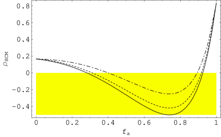
Figure 3: As Figure 1 but for the NPV parameter $\rho_{\scriptscriptstyle HCM}$ in the HCM. Shading indicates the region of NPV (i.e., $\rho_{\scriptscriptstyle HCM}<0$).

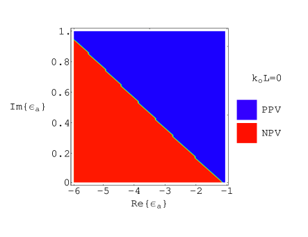
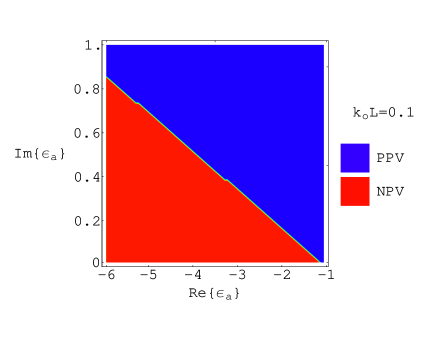
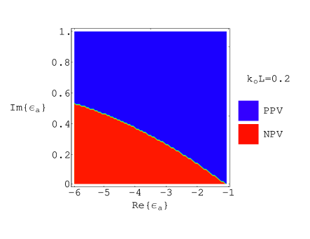
Figure 4: Regions of NPV and PPV, as estimated by the second–order SPFT in the long–wavelength approximation, in relation to $\mbox{Re}\left\{\epsilon_{a}\right\}\in(-6,-1)$ and $\mbox{Im}\left\{\epsilon_{a}\right\}\in(0,1)$. Whereas $k_{\scriptscriptstyle 0}L=0$, $0.1$, and $0.2$, the volume fraction is fixed at $f_{a}=0.3$. Other constituent material parameter values: $\mu_{a}=1.5+0.2i$, $\epsilon_{b}=-1.5+i$, and $\mu_{b}=2+1.2i$.

References

- [1] A. Lakhtakia, M.W. McCall and W.S. Weiglhofer, in: Introduction to Complex Mediums for Electromagnetics and Optics, W.S. Weiglhofer and A. Lakhtakia (eds.) (SPIE Press, Bellingham, WA, USA, 2003), pp.347–363.
- [2] S.A. Ramakrishna, Rep. Prog. Phys. 68, 449 (2005).
- [3] J.B. Pendry, Contemp. Phys. 45, 191 (2004).
- [4] R.A. Shelby, D.R. Smith and S. Schultz, Science 292, 77 (2001).
- [5] A. Grbic and G.V. Eleftheriades, J. Appl. Phys. 92, 5930 (2002).
- [6] A.A. Houck, J.B. Brock and I.L. Chuang, Phys. Rev. Lett. 90, 137401 (2003).
- [7] T.G. Mackay and A. Lakhtakia, Microwave Opt. Technol. Lett. 47, 313 (2005).
- [8] L. Ward, The Optical Constants of Bulk Materials and Films, 2nd ed. (Institute of Physics, Bristol, UK, 2000).
- [9] C.L. Holloway, E.F. Kuester, J. Baker–Jarvis and P. Kabos, IEEE Trans. Antennas Propagat. 51, 2596 (2003).
- [10] L. Jylhä, I. Kolmakov, S. Maslovski and S. Tretyakov, J. Appl. Phys. 99, 043102 (2006).
- [11] A. Lakhtakia and T.G. Mackay, AEÜ Int. J. Electron. Commun. 59, 348 (2005).
- [12] T.G. Mackay and A. Lakhtakia, Microwave Opt. Technol. Lett. 48, 709 (2005).
- [13] Yu. A. Ryzhov and V.V. Tamoikin, Radiophys. Quantum Electron. 14, 228 (1970).
- [14] U. Frisch, in: Probabilistic Methods in Applied Mathematics, Vol. 1, A.T. Bharucha–Reid (ed.) (Academic Press, London, UK, 1970), pp. 75–198.
- [15] L. Tsang and J.A. Kong, Radio Sci. 16, 303 (1981).
- [16] A. Stogryn, IEEE Trans. Antennas Propagat. 31, 985 (1983).
- [17] T.G. Mackay, A. Lakhtakia and W.S. Weiglhofer, Phys. Rev. E 62, 6052 (2000); erratum 63, 049901 (2001).
- [18] H.C. Chen, Theory of Electromagnetic Waves (McGraw–Hill, New York, NY, USA, 1983).
- [19] L. Tsang, J.A. Kong and R.W. Newton, IEEE Trans. Antennas Propagat. 30, 292 (1982).
- [20] T.G. Mackay, A. Lakhtakia and W.S. Weiglhofer, Opt. Commun. 197, 89 (2001).
- [21] R.A. Depine and A. Lakhtakia, Microwave Opt. Technol. Lett. 41, 315 (2004).
- [22] T.G. Mackay, Waves Random Media 14, 485 (2004); erratum (accepted for publication).