Essence of inviscid shear instability: a point view of vortex dynamics

Abstract

The essence of shear instability is fully revealed both mathematically and physically. A general sufficient and necessary stable criterion is obtained analytically within linear context. It is the analogue of Kelvin-Arnol’d theorem, i.e., the stable flow minimizes the kinetic energy associated with vorticity. Then the mechanism of shear instability is explored by combining the mechanisms of both Kelvin-Helmholtz instability (K-H instability) and resonance of waves. It requires both concentrated vortex and resonant waves for the instability. The waves, which have same phase speed with the concentrated vortex, have interactions with the vortex to trigger the instability. We call this mechanism as ”concentrated vortex instability”. The physical explanation of shear instability is also sketched. Finally, some useful criteria are derived from the theorem. These results would intrigue future works to investigate the other hydrodynamic instabilities.

The hydrodynamic instability is a fundamental problem in many fields, such as fluid dynamics, astrodynamics, oceanography, meteorology, etc. There are many kinds of hydrodynamic instabilities, e.g., shear instability due to velocity shear, thermal instability due to heating, viscous instability due to viscosity and centrifugal instability due to rotation, etc. Among them, the shear instability is the most important and the simplest one, which has been intensively explored (see Drazin and Reid (1981); Huerre and Rossi (1998); Criminale et al. (2003) and references therein). Both linear and nonlinear stabilities of shear flow have been considered, and some important conclusions have also be obtained from the investigations.

On the one hand, the nonlinear stability of shear flow has been investigated via variational principles. Kelvin Kelvin (1875) and Arnol’d Arnold (1965, 1969); Arnold and Khesin (1998) have developed variational principles for two-dimensional inviscid flow Saffman (1992). They showed that the steady flows are the stationary solutions of the energy $H$. And if the second variation $\delta^{2}H$ is definite, then the steady flow is nonlinearly stable. Moreover, Arnol’d proved that the flow is linearly stable provided that $\delta^{2}H$ is positive definite, and he also proved two nonlinear stability criteria Arnold (1969); Saffman (1992); Arnold and Khesin (1998); Vladimirov and Ilin (1999). However, $\delta^{2}H$ is always indefinite in sign, except for two special cases (see Vladimirov and Ilin (1999) and references therein). Though variational principle is indeed powerful, it is also inconvenient for real applications due to the lack of the explicit expressions in both $H$ and the stability criteria.

On the other hand, the linear stability of shear flow has also been investigated via Rayleigh’s equation. Within the linear context, there are three important general stability criteria, which are Rayleigh’s criterion Rayleigh (1880), Fjørtoft’s criterion Fjørtoft (1950) and Sun’s criterion Sun (2006a). As all the criteria have explicit expressions, they are more convenient in real applications, and are widely used in many fields. Based on the former investigations, Sun Sun (2006a) also pointed out that the flow is stable for Rayleigh’s quotient $I(f)>0$ (see Eq.(3) behind). However, the sufficient criterion for instability still lacks.

To understand the shear instability, some mechanisms were suggested. Among them, Kelvin-Helmholtz instability (K-H instability) is always taken as a prototype, which is physically explained as the instability of a sheet vortex Batchelor (1967). An another mechanism of instability is due to the resonance of waves Craik (1971); Butler and Farrell (1992); Baines and Mitsudera (1994); Staquet and Sommeria (2002); Criminale et al. (2003). Butler and Farrell Butler and Farrell (1992) clearly showed with numerical simulations that the resonance introduces an algebraic growth term into the temporal development of a disturbance. Baines and Mitsudera Baines and Mitsudera (1994) also used broken-line profile velocity as a prototype to explain the interaction of waves. Their explanation is so brilliant that it can explain why the instability occurs for a finite range of wavenumber and how the waves amplify each other. However, both mechanisms are independent of the basic flows, for that Kelvin-Helmholtz model deals only with vortex and resonance mechanism only considers the waves. Thus the relationships between those mechanisms and the shear flows are still covered.

Overview the former investigations, the essence of the shear instability is remained to be elucidated. Though $H$ is very important in variational principles, both the explicit expression and the meaning of it have not been revealed before. The connection between linear and nonlinear stability criteria should be retrieved explicitly. The relationships between instability mechanisms and the physical explanation for shear instability are needed. The aim of this letter is to fully reveal the essence of the shear instability by investigating the inviscid shear flows in a channel. And other instabilities in hydrodynamics may also be understood via the investigation here.

For the two-dimensional inviscid flows with the velocity of $U$, the vorticity $\xi=\nabla\times U$ is conserved along pathlines Batchelor (1967); Saffman (1992); Huerre and Rossi (1998):

$$\frac{d\xi}{dt}=\frac{\partial\xi}{\partial t}+(U\cdot\nabla)\xi=0.$$ (1)

Its linear disturbance reduces to Rayleigh’s equation provided the basic flow $U$ being parallel. Consider an shear flow with parallel horizontal velocity $U(y)$ in a channel, as shown in Fig.1. The amplitude of disturbed flow streamfunction $\psi$, namely $\phi$, satisfies Drazin and Reid (1981); Huerre and Rossi (1998); Criminale et al. (2003) :

$$(\phi^{\prime\prime}-k^{2}\phi)-\frac{U^{\prime\prime}}{U-c}\phi=0,$$ (2)

where $k$ is the nonnegative real wavenumber and $c=c_{r}+ic_{i}$ is the complex phase speed and double prime ^′′ denotes the second derivative with respect to $y$. The real part $c_{r}$ is the phase speed of wave, and $c_{i}\neq 0$ denotes instability. This equation is to be solved subject to homogeneous boundary conditions $\phi=0$ at $y=a,b$.

Consider that the velocity profile $U(y)$ has an inflection point $y_{s}$ at which $U^{\prime\prime}_{s}=U^{\prime\prime}(y_{s})=0$ and $U_{s}=U(y_{s})$. As Sun Sun (2006a) has pointed out, the following Rayleigh’s quotient $I(f)>0$ implies the flow is stable.

$$I(f)=\min_{\phi}\frac{\int_{a}^{b}[\,\|\phi^{\prime}\|^{2}+f(y)\|\phi\|^{2}\,]\,dy}{\int_{a}^{b}\|\phi\|^{2}}$$ (3)

where $f(y)=\frac{U^{\prime\prime}}{U-U_{s}}$. While if $I(f)<0$, then there is a neutral stable model with $k_{N}^{2}=-I(f)$ and $c_{r}=U_{s}$. Moreover, there are unstable modes with $c_{r}=U_{s}$ and $c_{i}\neq 0$ if $I(f)<0$ and $0\leq k<k_{N}$. This can also be proved by following the way by Tollmien Tollmien (1936), Friedrichs Friedrichs (1942); Drazin and Howard (1966); Drazin and Reid (1981) and Lin Lin (1955). Thus $I(f)=0$ means the flow is neutrally stable. And there is only one neutral mode with $k=0$ and $c_{r}=U_{s}$ in the flow. These conclusions can be summarized as a new theorem.

Tollmien-Fridrichs-Lin theorem: The flows are neutrally stable, if $I(f)=0$. The flows are stable and unstable for $I(f)>0$ and $I(f)<0$, respectively.

From the above proof, it is obvious that the shortwaves (e.g. $k\gg k_{N}$) are always more stable than longwaves (e.g. $k\ll k_{N}$) in the inviscid shear flows Drazin and Howard (1966); Sun (2006b). So the shear instability is due to long-wave instability, and the disturbances of shortwaves can be damped by the shear itself without any viscosity Sun (2006b).

As mentioned above, the linear stability criterion can be derived from the nonlinear one Arnold (1969). Moreover, the nonlinear stability criterion can also be obtained from the linear one. To illuminate this, the nonlinear criterion is retrieved explicitly via the above theorem, which is briefly proved as follows.

Similar to Arnol’d’s definition, the general energy $H$ here is defined as

$$H=\frac{1}{2}\int_{a}^{b}[\frac{1}{2}\|\nabla\Psi\|^{2}+h(\Psi)]dy$$ (4)

where $\Psi(y)$ is the streamfunction of the flow with $\frac{\partial\Psi}{\partial y}=U(y)-U_{s}$, and $h(\Psi)$ is a function of $\Psi$. The variation of $\delta H=0$ gives

$$\triangle\Psi=h^{\prime}(\Psi).$$ (5)

So Arnol’d’s variational principle is retrieved. The function $h=\|\nabla\Psi\|^{2}/2$ can also be solved from Eq.(5). The second variation $\delta^{2}H$ holds

$$\delta^{2}H=\frac{1}{4}\int_{a}^{b}[\|\nabla\psi\|^{2}+h^{\prime\prime}(\Psi)\psi^{2}]dy,$$ (6)

where $\psi$ denotes the variation $\delta\Psi$. Noting that $h^{\prime\prime}(\Psi)$ remains unknown, Arnol’d’s nonlinear criteria have not be extensively used. Fortunately, we can obtain the explicit expression of $h^{\prime\prime}(\Psi)$ here via the investigation on the linear stability criterion. For $\frac{\partial\Psi}{\partial y}=U-U_{s}$,

$$h^{\prime\prime}(\Psi)=\frac{dh^{\prime}}{d\Psi}=\frac{dh^{\prime}}{dy}\frac{dy}{d\Psi}=\frac{U^{\prime\prime}}{(U-U_{s})}=f(y).$$ (7)

As $h^{\prime\prime}(\Psi)$ is solved explicitly, $\delta^{2}H$ has an explicit expression, which is greatly helpful for real applications.

Let the streamfunction of the perturbation $\psi(x,y,t)=\phi(y)e^{i(kx-\omega t)}$, where $\omega$ is the frequency. The averages of $\|\nabla\psi\|^{2}$ and $\|\psi\|^{2}$ are $(\|\phi^{\prime}\|^{2}+k^{2}\|\phi\|^{2})/2$ and $\|\phi\|^{2}/2$ along the flow direction $x$, respectively. So Eq.(6) reduces to

$$\delta^{2}H=\frac{1}{8}\int_{a}^{b}[\|\phi^{\prime}\|^{2}+k^{2}\|\phi\|^{2}+f(y)\|\phi\|^{2}]dy.$$ (8)

The sign of $\delta^{2}H$ is then associated with $I(f)$ in Eq.(3). If $I(f)<0$, the second variation $\delta^{2}H$ can be both negative and positive, i.e., the stationary solution is a saddle point. And $I(f)>0$ implies $\delta^{2}H$ is positive definite and vice versa. So the stable flow has the minimum value of the total kinetic energy $H$. The physical meaning of $H$ can also be revealed, as the explicit expressions of $H$, $\frac{\partial\Psi}{\partial y}=U-U_{s}$ and $h^{\prime\prime}(\Psi)=f(y)$ are obtained.

First, according to the expressions, the velocity $U$ in vorticity conservation law Eq.(1) can be decomposed to two parts: the rotational flow $U-U_{s}$ and the irrotational advection flow $U_{s}$. The vorticity $\xi$ in Eq.(1) depends only on $U-U_{s}$, and $U_{s}$ is only advection velocity. Then $U-U_{s}$ and $U_{s}$ are associated with the dynamics and kinetics of the flow, respectively. Eq.(1) physically shows that the vorticity field is advected by $U_{s}$, which can also known from the conservation of vorticity in the inviscid flows. A similar example is the dynamics of vortex in the wake behind cylinder, where the vortices dominate the dynamics of the flow and they are advected by mean flow (see Fig.2 in Ponta and Aref (2002)). The decomposition of velocity may be useful in vortex dynamics, for that our investigation clearly shows that the dynamics of the flow is dominated by vorticity distribution.

Then the physical meaning of $H$ can also be understood from the above investigation. It is not $U$ but $U-U_{s}$ that is associated with the general energy $H$, so $H=\frac{1}{2}\int_{a}^{b}(U-U_{s})^{2}dy$ is not the total kinetic energy but the kinetic energy of flow with vorticity. Thus the stable steady states are always minimizing the kinetic energy of the flow associated with vorticity. This is also the reason why the flow with maximum vorticity might be unstable, as Fjørtoft’s criterion shows. We would like to restate it as a theorem and to name it after Kelvin Kelvin (1875) and Arnol’d Arnold (1969) for their contributions on this field Saffman (1992).

Kelvin-Arnol’d theorem: the stable flow minimizes the kinetic energy of flow associated with vorticity.

Both Tollmien-Fridrichs-Lin theorem and Kelvin-Arnol’d theorem are equivalent to the following simple principle Sun (2005): The flow is stable, if and only if all the disturbances with $c_{r}=U_{s}$ are neutrally stable.

We have obtained the sufficient and necessary conditions for instability, then the physical mechanism of instability can be understood from them. The following investigation will reveal that the essence of shear instability is due to the interaction between the ”concentrated vortex” and the corresponding resonant waves.

The concept of ”concentrated vortex” comes from Fjørtoft’s and Sun’s criteria, where the necessary conditions for instability require that the base vorticity must be concentrated enough Sun (2006a). We call it ”concentrated vortex” for latter convenience. The concentrated vortex is a general model of sheet vortex in the Kelvin-Helmholtz model, for that the sheet vortex can be recovered as the concentrated vortex $\xi(y_{s})\rightarrow\infty$ (see Vallis (2006) for a comprehensive discussion about the Kelvin-Helmholtz model and continued shear profiles). Then how the shear flow becomes unstable, if there is a concentrated vortex? As the sufficient condition for instability is $I(f)<0$, the normal modes in the regime of $0\leq k<k_{N}$ with $c_{r}=U_{s}$ are unstable. They are stationary or standing waves, comparing to the velocity at inflection point. So that the shear instability is due to the disturbance of concentrated vortex by the standing waves with $c_{r}=U_{s}$. In this case, the resonance mechanism is valid. The interaction waves propagate at the same speed with the concentrated vortex, so that they are locked together and amplified by simple advection Baines and Mitsudera (1994). In short, the disturbances on concentrated vortex is amplified like that in Kelvin-Helmholtz model.

This instability mechanism combines both K-H instability and resonance mechanism. Physically, the standing waves (with $c_{r}=U_{s}$) can interact with the concentrated vortex, so they can trigger instability in the flows. While the travelling waves (with $c_{r}\neq U_{s}$) have no interaction with the concentrated vortex, so that they can not trigger instability in the flows. This is the mechanism of shear instability. As pointed out above, the shear instability is due to long-wave instability. If the longwaves are unstable, they can obtain the energy from background flows. In this way, the energy within small scales transfer to and concentrate on large scales. In this way, the shear instability itself provides a mechanism to inverse energy cascade and to maintain the large structures or coherent structures in the complex flows.

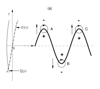
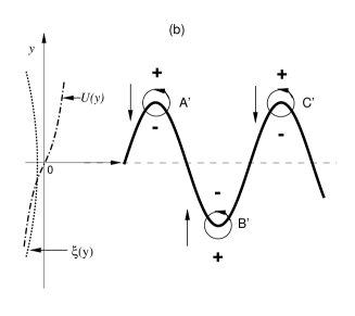
Figure 1: Sketch of shear instability: physical interpretation. Left parts depict the profiles of velocity $U(y)$ and vorticity $\xi(y)$, right ones depict the disturbance of vorticities. The unstable veloctiy profile $U(y)$ has a local maximum in vorticity $\xi(y)$ (a). If the vortices (A, B and C) disturbed from their original positions (dashed line) to new places (solid curve), they will be taken away from their original positions due to pressure difference. The stable veloctiy profile $U(y)$ has a local minimum in vorticity $\xi(y)$ (b). The disturbed vortices (A’, B’ and C’) will be brought back to their original positions due to pressure difference.

To illuminate the mechanism of shear instability, a physical diagram is also presented here by following the way of interpreting the K-H instability Batchelor (1967). Fig.1 sketches the mechanism of shear instability in terms of wave disturbances of vortices. The mean velocity profile $U(y)$ has an inflection point at $y_{s}=0$ with $U_{s}=0$, and the corresponding vorticity is $\xi(y)=-U^{\prime}(y)$. There is a local maximum at $y_{s}$ in the unstable vorticity profile in Fig.1a. According to Eq.(1), the vorticity is conserved in the inviscid flows. If the vortices at the local maximum (A, B and C) are sinusoidally disturbed from their original positions (dashed line) to new places (solid curve), they have negative vorticities with respect to the undisturbed ones. The vortices will induce cyclone flows around them in consequence. The flows around the vortices become faster (slower) in the upper (lower) of vortex A referred to the basic flow $U(y)$. The pressures at upper and lower decrease (indicated by - signs) and increase (indicated by + signs) according to Bernoulli’s theorem, respectively. Then vortex A gets a upward acceleration due to the disturbed pressure difference as the uparrow shows. This tends to take the vortex away from its original position, so the flow is unstable. On the other hand, Fig.1b depicts the disturbances in a stable velocity profile, where a local minimum is in the vorticity profile. The disturbed vortices have positive vorticities with respect to the undisturbed ones. The vortices will induce anticyclone flows around them in consequence. So vortex A’ get a downward acceleration due to the disturbed pressure difference as the downarrow shows. This tends to bring the vortex back from its original position, so the flow is stable. In this interpretation, the advection of $U_{s}$ is independent of the shear instability, only the flow field of $U-U_{s}$ and the corresponding vorticity $\xi$ are the dominations. The unstable disturbances in Fig 1 have $c_{r}=U_{s}$, which consists with the former discussions. This physically explains why the maximum and minimum vorticities have different stable aspects.

Though Tollmien-Fridrichs-Lin theorem is a sufficient and necessary condition for stability, the unknown $\phi$ in the theorem restricts its application. So some simple criteria may be more useful. For the parallel flows within interval $a<y<b$, there are two simple criteria.

Corollary 1: The flow is stable for $f(y)>-(\frac{\pi}{b-a})^{2}$ Sun (2005, 2006a).

Corollary 2: The flow is unstable for $f(y)<-(\frac{\pi}{b-a})^{2}$ Sun (2005).

In summary, the general stability and instability criteria are obtained for inviscid parallel flow. And the criterion is associated with a minimum value of energy, which shows the relationship between linear and nonlinear stability criteria. Then the mechanism of shear instability is investigated, which is explained as the resonance of standing waves with the concentrated vortex at $c_{r}=U_{s}$. A physical explanation is also sketched. Finally, some useful criteria are given. In general, these criteria will lead future works to investigate other instabilities in hydrodynamics.

The work was original from author’s dream of understanding the mechanism of instability in the year 2000, when the author was a graduated student and learned the course of hydrodynamics stability by Prof. Yin X-Y at USTC.

References

- Drazin and Reid (1981) P. G. Drazin and W. H. Reid, Hydrodynamic Stability (Cambridge University Press, 1981).
- Huerre and Rossi (1998) P. Huerre and M. Rossi, in Hydrodynamics and nonlinear instabilities, edited by C. Godrèche and P. Manneville (Cambridge University Press, Cambridge, 1998).
- Criminale et al. (2003) W. O. Criminale, T. L. Jackson, and R. D. Joslin, Theory and computation of hydrodynamic stability (Cambridge University Press, Cambridge, U.K., 2003).
- Kelvin (1875) L. Kelvin, Collected works IV, 115 (1875).
- Arnold (1965) V. I. Arnold, J. Applied Math. and Mechan. 29(5), 1002 (1965).
- Arnold (1969) V. I. Arnold, Amer. Math. Soc. Transl. 19, 267 (1969).
- Arnold and Khesin (1998) V. Arnold and B. Khesin, Topological methods in hydrodynamics (Springer-Verlag, 1998).
- Saffman (1992) P. G. Saffman, Vortex Dynamics (Cambridge University Press, Cambridge, U.K., 1992).
- Vladimirov and Ilin (1999) V. A. Vladimirov and K. I. Ilin, in The Arnoldfest: Proceedings of a Conference in Honour of V.I. Arnold for His Sixtieth Birthday, edited by E. Bierstone, B. Khesin, A. Khovanskii, and J. E. Marsden (American Mathematical Society, 1999), pp. 471–495.
- Rayleigh (1880) L. Rayleigh, Proc. London Math. Soc. 11, 57 (1880).
- Fjørtoft (1950) R. Fjørtoft, Geofysiske Publikasjoner 17, 1 (1950).
- Sun (2006a) L. Sun, arXiv:physics/0601043 (2006a).
- Batchelor (1967) G. K. Batchelor, An Introduction to Fluid Dynamics (Cambridge University Press, Cambridge, U. K., 1967).
- Craik (1971) Craik, J. Fluid Mech. 50, 393 (1971).
- Butler and Farrell (1992) K. M. Butler and B. F. Farrell, Phys. Fluids A 4, 1637 (1992).
- Baines and Mitsudera (1994) P. Baines and H. Mitsudera, J. Fluid Mech. 276, 327 (1994).
- Staquet and Sommeria (2002) C. Staquet and J. Sommeria, Ann. Rev. Fluid Mech. 34, 559 (2002).
- Tollmien (1936) W. Tollmien, Tech. Rep. NACA TM-792, NACA (1936).
- Friedrichs (1942) K. O. Friedrichs, Fluid dynamics (Brown University, Providence, Rhode Island, 1942).
- Drazin and Howard (1966) P. G. Drazin and L. Howard, in Advances in applied mechanics, edited by G. G. Chernyi (Academic Press, New York, 1966), vol. 9, pp. 1–81.
- Lin (1955) C. C. Lin, The Theory of Hydrodynamic Stability (Cambridge University Press, London, UK, 1955).
- Sun (2006b) L. Sun, arXiv:physics/0601112 (2006b).
- Ponta and Aref (2002) F. L. Ponta and H. Aref, Phys. Rev. Lett. 93(8), 084501 (2002).
- Sun (2005) L. Sun, arXiv:physics/0512208 (2005).
- Vallis (2006) G. K. Vallis, Atmospheric and Oceanic Fluid Dynamics (Cambridge University Press, Cambridge, U. K., 2006), doi:10.2277/0521849691.