International Journal of Simulation and Process Modelling 2, Nos. 1/2, pp. 67-79 (2006) [a special issue on “Mathematical Modelling and Simulation for Industrial Applications”; Editors: S. Olariu (USA), B. B. Sanugi (Malaysia) and S. Salleh (Malaysia)].

An Extended Interpretation of the Thermodynamic Theory Including
an Additional Energy Associated
with a Decrease in Mass

Volodymyr Krasnoholovets¹ and Jean-Louis Tane²

¹Institute for Basic Research, 90 East Winds Court, Palm Harbor, FL 34683, U.S.A.,  v_kras@yahoo.com

²Formerly with the Department of Geology, Joseph Fourier University, Grenoble, France,   TaneJL@aol.com

Abstract. Although its practical efficiency is unquestionable, the thermodynamic tool presents a slight inconsistency from the theoretical point of view. After exposing arguments, which explain this opinion, a suggestion is put forward to solve the problem. It consists of linking the mass-energy relation $\pm\Delta{\kern 1.0pt}m{\kern 1.0pt}{\kern 1.0pt}c^{2}$ to the laws of thermodynamics. This combination results in a clarification of the theory and opens a bridge between thermodynamics and gravitation. It is shown that the submicroscopic consideration, which is based on the cellular concept of the real physical space when the space is treated as the tessellation lattice, indeed strongly supports the idea of a variation in mass in thermodynamic processes.

Key words: thermodynamics, entropy, mass, matter waves, inertons, gravitation, relativity, quantum mechanics

PACS: 01.55.+b; 03.65.Ta; 03.75.-b; 04.60.-m; 05.70.-a

Biographical notes: Dr. Volodymyr Krasnoholovets is senior scientist at the Institute of Physics, National Academy of Sciences of Ukraine, and Professor of the Institute for Basic Research, Florida, USA. His research touches conventional, fundamental and applied physics. The most internationally known results were obtained in the physics of hydrogen-bonded systems and the fundamental physics. In the realm of the fundamentals, jointly with late Professor Michel Bounias (Université d’Avignon, France) they constructed a detailed mathematical theory of the real physical space that appears as a tessellation of primary topological balls. The theory has already received an international recognition, first of all among mathematicians. The theory strongly supports Krasnoholovets submicroscopic mechanics developed in the real space on the Planck scale $\approx 10^{-35}$ m which is easily transformed to the abstract formalism of conventional quantum mechanics constructed on the atomic scale, $\approx 10^{-10}$ m. For more details see his web site http://www.inerton.kiev.ua.

Dr. Jean-Louis Tane is a retired scientist whose speciality is geology that he taught during more than thirty years at Joseph Fourier University, Grenoble, France, and during three years at the University of Marrakech, Morocco. Most of his papers deal with geologic topics, particularly the problem of the origin of spilitic rocks, yet one of his courses concerned the use of thermodynamics in geochemistry. His interest for physics has been confirmed recently, by the writing of several papers suggesting a link between thermodynamics and relativity. They have been published, between 2000 and 2004 in the Journal of Theoretics.

1. Statement of the problem

Following typical thermodynamic courses (see, e.g. Refs. [1-4]), let us consider the experimental context of an isolated system composed of two parts separated by a mobile piston. We assume that part 1 contains a gas whose initial pressure is ${P}_{1}$ while part 2 is a vacuum. If the piston, previously locked, is released, the gas expands into the whole system and the thermodynamic interpretation usually given to the process is based on the two following equations

$${dU=dQ+dW},$$ (1)

$${dU=TdS-PdV},$$ (2)

whose significations and mutual relations are well-known. A more conventional writing of eq. (1) would be ${dU=\delta Q+\delta W}$, but the simplified and general transcription adopted here has no influence on the discussion presented below. Note that the usual reasoning tend to focus attention on the gas for which it is successively written:

${dQ}=0$ (since the gas cannot exchange heat with the vacuum);

${dW}=0$ (since, by definition, $dW=-P_{\rm ext}dV$, where $P_{\rm ext}$ is the pressure external to  the gas, i.e. the pressure $P_{\rm ext}=0$ of the vacuum and $dV$ the change in volume of the gas);

${dU}=0$ (being the sum ${dQ+dW}$);

then owing to the equality $dU=0$ we have $dS=(P/T)dV$ where the three quantities P, T and ${dV}$ are positive and hence ${dS}$ is positive too.

On this basis, it is implicitly admitted that the relation $dU=0$ is true not only for the gas, but equally for the whole system defined as isolated. It is precisely upon this point that an important and interesting problem arises.

To be rapidly convinced of this reality, let us imagine an experimental context identical to the one just considered, except that instead of being vacuum, part 2 would contain a gas whose initial pressure is $P_{2}$. In such a case, applying equation $dW=-P_{\rm ext}{dV}$ to part 1 and part 2 leads to the doublet of equations:

$${dW}_{1}={-P}_{2}{\kern 1.0pt}dV_{1},$$

$${dW}_{2}={-P}_{1}{dV}_{2}.$$

Noting that ${dV}_{2}={-dV}_{1}$, we get for the whole system

$$dW=dV_{1}(P_{1}-{P}_{2}).$$ (3)

Since dV1 is positive when $P_{1}>P_{2}$ and negative when $P_{1}<P_{2}$, equation (3) shows that $dW$ is always positive and reaches the value zero only when ${P}_{1}={P}_{2}$. In other words, we are facing the fact that the disappearance of the pressure gradient within the system is accompanied by an additional energy whose origin in inside this system.

The process examined just before (expansion of a gas in vacuum) corresponds to the particular case for which ${P}_{2}=0$ in equation (3), so that ${dW}$ has a positive value, not a zero value as previously recalled and classically accepted. This is the sign that the vacuum plays an important role in the calculation. When equation ${dW}={-P}_{\rm ext}{dV}$ is applied to it, ${P}_{\rm ext}$ corresponds to the pressure of the gas and ${dV}$ to the decreasing volume of the vacuum, which can be noted ${dV}_{\rm vacuum}$. Accordingly, $dW_{\rm vacuum}$ has a positive value and represents at the same time ${dW}_{\rm system}$, given that ${dW}_{\rm gas}$ is zero.

Transposing these results in equation (1), and applying it to the whole system, we see that the only condition to obtain ${dU}_{\rm system}=0$ is that ${dQ}_{\rm system}$ should be negative. Such a condition is not compatible with one of the fundamental laws of thermodynamics (sometimes called the law of heat exchange), which relies on the idea that an exchange of heat between two parts 1 and 2 of an isolated system is described by the relation ${dQ}_{2}={-dQ}_{1}$. At the scale of the whole system, this relation leads to the conclusion

$$dQ=dQ_{1}+dQ_{2}=0.$$ (4)

where ${dQ}_{1}$ and ${dQ}_{2}$ represent the change in heat for the gas and the vacuum.

As will be explained further, it is highly probable that the true value of ${dQ}$ is not zero but positive. At the present stage of the discussion, combining the idea that ${dQ}$ is not negative with the fact, already noted, that ${dW}$ is positive provides a sufficient condition to conclude that ${dU}$ is itself positive. Hence, there is really something not clear in the usual conception of thermodynamics, which is based on the idea that the internal energy change ${dU}$ for an isolated system obeys the double equation

$$dU=dQ+dW=0.$$

2. A suggestion to solve the problem

We have seen in the section 1 that the disappearance of the pressure gradient within an isolated system is accompanied by a creation of energy inside this system. Previously we [5-9] preliminary analyzed of the problem and proposed a way to its solution. Now let us elucidate all the aspects of the problem in detail.

We can give to this energy created inside the system studied the designation ${dW}_{\rm int}$, in order to distinguish it from the energy ${dW}_{\rm ext}$ that (in the more general case of a non isolated system) corresponds to the exchange of work between the system and its surroundings. With these designations, ${dW}$ takes the signification

$${dW=dW}_{\rm ext}+{dW}_{\rm int}.$$ (5)

The condition ${dW}_{\rm ext}=0$ means that the system is isolated (in the sense classically given to this concept in thermodynamics). The condition ${dW}_{\rm int}=0$ means that there is no pressure gradient (i.e. no irreversibility of pressure) within this system. Contrary to ${dW}_{\rm int}$, which, as already seen, obeys the relation

$${dW}_{\rm int}\geq 0.$$ (6)

The value of $dW_{\rm ext}$ can be positive or negative, depending on whether the system receives work or gives work in its exchanges with the surroundings.

If the system we are considering is not isolated but only closed, the work ${dW}$ exchanged with its surroundings (and whose precise designation is ${dW}_{\rm ext}$) is given, as recalled above, by the classical expression $dW=-P_{\rm ext}{\kern 1.0pt}{dW}$. If we are under conditions of reversibility, i.e. if ${P}_{\rm ext}={P}_{\rm int}$, this relation becomes $dW=-P_{\rm int}{dV}$. Observing that ${P}_{\rm ext}$ can always be written ${P}_{\rm ext}={-P}_{\rm int}+{P}_{\rm int}+{P}_{\rm ext}$, we get the general; expression

$${dW=-P}_{\rm int}{dV}-{(P}_{\rm ext}{-P}_{\rm int}{)}{dV},$$ (7)

which means

$${dW}_{\rm irr}={dW}_{\rm rev}+\textit{dW}_{\rm int},$$ (8)

that is

$${dW}_{\rm irr}={dW}_{\rm ext}+{dW}_{\rm int}.$$ (9)

Each term of eqs. (8) and (9) has the same value and signification as the corresponding term of equation (7). An important point to be noted is that ${dW}_{\rm ext}={dW}_{\rm rev}$.

As concerns the exchanges of heat and their relations with the concept of entropy, the usual thermodynamic tool is given by the well-known expression

$$dS\geq dQ/T_{\rm ext},$$

which can be represented in the form

$${dS=dQ/T}_{\rm ext}+{dS}_{\rm int}.$$ (10)

To be coherent with the reasoning previously adopted, eq. (10), which has the dimensionality of entropy, needs to be converted in an equation having the dimensionality of energy, i.e.

$${T}_{\rm ext}dS=dQ+T_{\rm ext}dS_{\rm int}.$$ (11)

whose signification is

$$dQ=dQ_{\rm ext}+{dQ}_{\rm int},$$ (12)

that is

$${dQ}_{\rm irr}={dQ}_{\rm rev}+{dQ}_{\rm int}.$$ (13)

Each term of eqs. (12) and (13) has the same value and signification as the corresponding term of eq. (11). As well as we have observed that ${dW}_{\rm ext}={dW}_{\rm rev}$ we see here that ${dQ}_{\rm ext}={dQ}_{\rm rev}$ but this last equality is not a novelty. In the usual conception of the thermodynamic theory, it is an implicit equation whose integration leads to eq. (21) that will be used further.

In the same manner as we have introduced a difference between ${dW}_{\rm ext}$ and ${dW}_{\rm int}$ in eq. (5) and a difference between ${dQ}_{\rm ext}$ and ${dQ}_{\rm int}$ in eq. (12), we now easily conceive that there is a difference between ${dU}_{\rm ext}$ and ${dU}_{\rm int}$. It can be expressed through the general equation

$${dU=dU}_{\rm ext}+dU_{\rm int},$$ (14)

which can be better written (as explained hereafter) in the form

$$dU^{*}=dU_{\rm ext}+dU_{\rm int}$$ (15)

whose meaning is

$${dU}_{\rm irr}={dU}_{\rm rev}+{dU}_{\rm int}.$$ (16)

For reasons of homogeneity with eq. (15), equations (5) and (12) can be written respectively

$$dW^{*}=dW_{\rm ext}+{dW}_{\rm int}$$

and

$$dQ^{*}=dQ_{\rm ext}+dQ_{\rm int}.$$ (17)

In conventional thermodynamics, ${dU}_{\rm ext}$ is generally noted ${dU}$. It is to avoid the risk of an additional confusion that the sum ${dU}_{\rm ext}+{dU}_{\rm int}$ has been noted ${dU^{*}}$ (and not simply ${dU}$) in eq. (15). The conceptual difficulty which is often encountered in learning (and teaching) thermodynamics comes from the fact that ${dU}_{\rm int}$ is not recognized as an energy, so that ${dU^{*}}$ and ${dU}_{\rm ext}$ are not differentiated. Consequently, they are expressed through the same designation ${dU}$ with the drawback evoked above.

We have just recalled that the term usually noted ${dU}$ in thermodynamics corresponds to the one noted ${dU}_{\rm ext}$ in eq. (15). Concerning the energetic quantity ${dU}_{\rm int}$ and given that it is generated within the system, there is no other solution to explain its origin as that of a correlative decrease in mass, according to the Einstein mass-energy relation. Since this relation was not known when the laws of thermodynamics have been stated, we easily conceive that it was not evident for their authors to imagine such a possibility, all the more that the decrease in mass is generally much too small to be experimentally detectable.

The practical and well-known efficiency of the thermodynamic tool is evidently due to the fact that although not identified as an energy, the term ${dU}_{\rm int}$ is nevertheless taken into account through the concept of the internal component of entropy, usually noted ${dS}_{\rm int}$. We have to note that being a physical reality, ${dU}_{\rm int}$ is not easy to eliminate. It is certainly for this reason that the art of playing thermodynamics often looks like an acrobatic feat whose objective is to convert ${dU}_{\rm int}$ into ${dS}_{\rm int}$ everywhere it appears. For instance, at the study of anomalies in water, we [10,11] were forced to introduce an additional correction to the Gibbs potential called “the change of the Gibbs potential associated with intermolecular interaction (or the configuration potential)” $G_{\rm in.in.}=(C_{\rm p}-S)\Delta T$; this potential definitely introduced a correction to the entropy $S$ of the water system studied.

On the other hand, let us now look at the Einstein mass-energy relation that classically is presented through the expression $E=mc^{{\kern 0.7pt}2}$ where $c$ is the speed of light. In the differential form its becomes

$$dE=c^{2}dm,$$

which would be preferably written for our case as $dE=-c^{{\kern 0.7pt}2}{dm}$, since ${dE}$ is positive when ${dm}$ is negative and conversely. Transposed in the language of thermodynamics and taking into account the term ${dU}_{\rm int}$ previously explained, this expression becomes

$${dU}_{\rm int}=-c^{{\kern 0.7pt}2}{dm}.$$ (18)

We have seen above that ${dU}_{\rm int}$ is the energy created within a system, due to the disappearance of an internal gradient that is of an internal irreversibility. Combining this data with the observation, evidenced for a long time by scientists, that every kind of irreversibility generates heat, both the term ${dW}_{\rm int}$ of eq. (5) and the term ${dQ}_{\rm int}$ of eq. (13) can appear as being heat.

The great difference between the theory suggested here and the classical one lies in the origin of the heat, which is linked to irreversibility. In conventional thermodynamics, this heat is considered as coming from the fact that the energy received by the system, from its surroundings, is partly transformed into thermal energy. In our theory, the energetic quantity ${dU}_{\rm int}$ is considered as resulting from a partial disintegration of mass inside the system. For a better understanding of this difference, a practical and numerical example is examined below.

3. A numerical application of the suggested theory

Let us consider an isolated system composed of two parts 1 and 2, each of them containing liquid water. We suppose that the initial temperature ${T}_{1}$ of part 1 is 293 K (20^∘ C) and that the initial temperature ${T}_{2}$ of part 2 is 333 K (60^∘ C). We know that the evolution of the system consists of an irreversible exchange of heat between the two parts, until they reach the same final temperature $T_{\rm f}$. We also know that T_f is given by the relation

$$T_{\rm f}=(C_{1}T_{1}+C_{2}T_{2})/(C_{1}+C_{2})$$ (19)

where ${C}_{1}$ and $C_{2}$ are the heat capacities of part 1 and part 2, respectively. To simplify the calculation without reducing its interest, we can assume that the mass of water is the same in each part and choose it in such a way that $C_{1}={C}_{2}=1$ J. Since C = 4.18 J for one gram of water, the mass we have to consider is $1/(4.18)=0.223$ [g]. Knowing that liquid water is a condensed form of water, we can also note that C designates indifferently $C_{v}$ and $C_{\rm p}$ (whose values are quite equal in such a case) and that we make an acceptable approximation in considering that ${C}$ does not vary significantly with temperature.

Admitting these considerations, the difference between the classical interpretation and the one suggested presently is the following.

3.1. The classical interpretation

Eq. (19) gives

$${T}_{\rm f}=(1\times 293+1\times 333)/(1+1)K=313{\rm K}.$$ (20)

From the general relation

$$\Delta Q=C\times(T_{\rm f}-T_{\rm i})$$ (21)

where $T_{i}$ means $T_{\rm initial}$ and having, in the present case, $\Delta U=\Delta Q$ (since $\Delta W=0$),

we obtain

$\Delta$ U₁ = $\Delta$Q₁ = 1 $\times$ (313 - 293) J = 20 J,

$\Delta$ U₂ = $\Delta$Q₂ = 1 $\times$ (313 - 333) J = - 20 J

so that, for the whole system

$\Delta$ U = $\Delta$Q = $\Delta$U₁ + $\Delta$U₂= 0.

Concerning the entropy change, the general equation is

$$\Delta{\kern 1.0pt}{\kern 1.0pt}S=\int\limits_{T_{1}}^{T_{2}}{\frac{{C}}{{T}}dT},$$ (22)

which gives

$\Delta S_{1}=\ln(313/293)=0.066030$ JK^-1,

$\Delta{S}_{2}=\ln(313/333)=-0.061939{\kern 2.0pt}{\rm JK}^{-1}$

so that, for the whole system:

$\Delta{S}=0.066030{\kern 2.0pt}{\rm JK}^{-1}-0.061939{\kern 2.0pt}{\rm JK}^{-1}=0.00409{\kern 2.0pt}{\rm JK}^{-1}$.

The important point to keep in mind is that $\Delta U$ is zero, while $\Delta S$ is positive.

3.2. The new suggested interpretation

By integration, eq. (11) leads to an expression, which can be written

$$T_{\rm ext}^{\ast}\Delta S=\Delta{Q+T}_{\rm ext}^{\ast}\Delta S_{\rm int},$$ (23)

whose meaning is

$$\Delta U^{\ast}=\Delta U_{\rm ext}+\Delta U_{\rm int}.$$

In eq. (23), $T_{\rm ext}^{\ast}$ represents the average external temperature that can be calculated as follows:

for part 1, its value is $T_{\rm ext}^{\ast}=T_{2}^{\ast}=\Delta Q_{2}/\Delta S_{2}=-20/(-0.061939)$ K = 322.89 K,

for part 2, its value is $T_{\rm ext}^{\ast}=T_{1}^{\ast}=\Delta Q_{1}/\Delta S_{1}=20/(0.066030)$ K = 302.89 K.

Contrary to $T_{1}$ and $T_{2}$, which are varying both in space and in time, $T_{1}^{\ast}$ and $T_{2}^{\ast}$ can be seen as space-time parameters, whose values are constant for the process we are considering. In a more general way, this peculiarity appears as a characteristic of $T_{\rm ext}^{\ast}$.

The terms $\Delta Q_{1}$, $\Delta Q_{2}$, $\Delta S_{1}$ and $\Delta S_{2}$ having the numerical values already calculated in section 3.1, when applying eq. (23) to part 1 and part 2 we get successively

for part 1:

$\Delta U^{\ast}_{1}=T_{\rm ext2}^{\ast}\Delta S_{1}=322.89\times 0.066030$ J = 21.32 J,

so that:

$\Delta U_{\rm int1}=\Delta U^{\ast}_{1}-\Delta U_{\rm ext1}=21.32$ J - 20 J = 1.32 J;

for part 2:

$\Delta U^{\ast}_{2}=T_{\rm ext1}^{\ast}\Delta S_{2}=302.89\times(-0.061939)$ J = - 18.76 J,

so that:

$\Delta U_{\rm int2}=\Delta U_{2}^{\ast}-\Delta U_{\rm ext2}=-18.76$ J - (- 20) J = 1.24 J;

for the whole system:

$\Delta U_{\rm int}=\Delta U_{\rm int1}+\Delta U_{\rm int2}=1.32$ J + 1.24 J = 2.56 J,

$\Delta U_{\rm ext}=\Delta U_{\rm ext1}+\Delta U_{\rm ext2}=20$ J $-{\kern 2.0pt}20$ J = 0,

so that

$\Delta U^{\ast}=\Delta U_{\rm ext}+\Delta U_{\rm int}$, i.e. $\Delta U^{\ast}=0$ J + 2.56 J = 2.56 J.

The essential point is that the value $\Delta U_{\rm ext}=0$ corresponds to the fact that the whole system is defined as isolated.

The value $\Delta U_{\rm int}>0$ corresponds to the fact that the evolution of this system (disappearance of an internal temperature gradient) is accompanied by an increase in energy whose value is 2.56 J and whose corresponding decrease in mass (according to the Einstein mass-energy relation) is

$$d{\kern 1.0pt}m=-2.56{\kern 1.0pt}/\left({3\times 10^{8}}\right)^{2}\;{\rm kg}=-2.84\times 10^{-17}{\kern 3.0pt}{\rm kg}.$$ (24)

Although this latter value is evidently too small to be detectable experimentally, it appears as the logic inference of the reasoning adopted.

4. The concept of free energy in the suggested theory

The concept of free energy, introduced by Gibbs, is of great usefulness in the thermodynamic study of chemical reactions. It is generally noted G and defined by the well-known equation

$$G=U+PV-TS$$ (25)

whose differential form is

$$dG=dU+d(PV-TS)$$ (26)

The point to be careful with when considering $G$ in the light of the new suggested theory is that ${dU}$, in eq. (26), corresponds to $dU_{\rm ext}$ that can itself be written indifferently as

$$dU_{\rm ext}=T_{\rm int}^{\ast}dS-P_{\rm int}^{\ast}dV$$ (27)

whose meaning is $dU_{\rm ext}=dU_{\rm reversible}$, or as

$$dU_{\rm ext}=T_{\rm ext}^{\ast}dS-P_{\rm ext}^{\ast}dV+c^{2}dm$$ (28)

whose meaning is

$$dU_{\rm ext}=dU^{\ast}-dU_{\rm int},\ \$$

i.e.

$$dU_{\rm ext}=dU_{\rm irr}-dU_{\rm int},$$

so that

$$dU_{\rm ext}=dU_{\rm rev}.\ \ \qquad$$

Thus we see that equation (28) is really coherent with eq. (27).

Taking into account these considerations, the whole meaning of eq. (26) can itself be understood through two equivalent interpretations:

4.1. The first interpretation

$$dG=T_{\rm int}^{\ast}dS-P_{\rm int}^{\ast}dV+d(PV-TS),$$ (29)

that is

$$dG=T_{\rm int}^{\ast}dS-P_{\rm int}^{\ast}dV+P_{\rm ext}^{\ast}dV+VdP_{\rm ext}^{\ast}-T_{\rm ext}^{\ast}dS-SdT_{\rm ext}$$

where $P_{\rm ext}$ and $T_{\rm ext}^{\ast}$ are constant (as already seen for $T_{\rm ext}^{\ast}$ in the section 3.2), so that $dT_{\rm ext}^{\ast}=0$ and $dP_{\rm ext}^{\ast}=0$. Consequently,

$$dG=(T_{\rm int}^{\ast}-T_{\rm ext}^{\ast}){\kern 1.0pt}dS+(P_{\rm ext}^{\ast}-P_{\rm int}^{\ast}){\kern 1.0pt}dV.$$ (30)

4.2. The second interpretation

The second interpretation is equivalent to the first one, but using $dU_{\rm ext}$ as defined by equation (28)

$$dG=T_{\rm ext}^{\ast}{\kern 1.0pt}dS-P_{\rm ext}^{\ast}{\kern 1.0pt}dV+c^{2}dm+d(PV-TS),$$ (31)

which (after the same treatment as that already done), is reduced to

$$dG=c^{2}dm.$$ (32)

Both equations are the same but the first transcription gives the formula to calculate $dG$ (29), while the second shows that $dG$ is correlated to a change in mass (32).

For a practical example of the use of these equations, let us come back to the exchange of heat between the two parts of the isolated system previously considered and to the interpretation presented in the section 3.2.

We are in a situation for which ${dV}$ is negligible, so that eq. (30) is reduced to

$$dG=(T_{\rm int}^{\ast}-T_{\rm ext}^{\ast}){\kern 1.0pt}dS.$$ (33)

Having noted above that $T_{\rm int}^{\ast}$ and $T_{\rm ext}^{\ast}$ are constants (referring to the process we are considering), the difference $T_{\rm int}^{\ast}-T_{\rm ext}^{\ast}$ is a constant too and, consequently, the integration of eq. (33) leads to

$$\Delta G=(T_{\rm int}^{\ast}-T_{\rm ext}^{\ast})\Delta S.$$ (34)

By applying eq. (34) to part 1 and part 2 successively, we get

$\Delta G_{1}=(302.89-322.89)\times 0.066030\ {\rm J}=-1.32\ {\rm J}$,

$\Delta G_{2}=(322.89-302.89)\times(-0.061939)\ {\rm J}=-1.24\ {\rm J}$,

so that, for the whole system, $\Delta G=\Delta G_{1}+\Delta G_{2}=-2.56$ J.

This result being the same (with an inversion of sign) as the one obtained in the section 3.2, we see that $\Delta G$ is effectively equivalent to - $\Delta U_{\rm int}$.

In the case of a chemical reaction, the negative value of $\Delta G$ corresponds to the disappearance, within the system, of a gradient in chemical potential. This peculiarity is a well-known data of the classical theory. The complementary information we obtain now is that the negative value of $\Delta G$ is accompanied by a decrease in mass.

The fact that conventional thermodynamics does not take into account the decrease in mass, which is linked to a chemical reaction, is probably the reason why it is not of common use in the study of nuclear reactions, which are effectively characterized by a change in mass. It seems that this difficulty disappears when the enlarged conception suggested here is substituted to the classical one.

After this preliminary consideration based on macroscopic thermodynamics, we will now examine the problem from the submicroscopic point of view.

5. Submicroscopic consideration

5.1. Space structure and quantum mechanics

Let us turn now to a microscopic consideration of a dynamic system. What has to be proved is the realistic mass exchange between the system studied and the ambient space. Obviously orthodox quantum mechanics cannot solve the problem, because it treats mass of a quantum system as an invariable classical parameter. At the same time relativistic experiments demonstrate that the mass is not a constant but changes with the system’s velocity. This means that something is wrong in our comprehension of the fundamentals, namely: There is no any connection between conventional quantum physics and relativity.

Very recently a rigorous mathematical theory of the real physical space has been developed by Bounias and Krasnoholovets [12-14]. The theory shows that the real space represents a mathematical lattice, called the tessellattice, packing with elementary cells whose size can be estimated as the Planck one, $\sim$ 10^-35 m. The tessellattice represents a degenerate space-time, i.e. in this case all cells (in other words, balls) are degenerated.

A particled cell provides a formalism describing the elementary particles proposed in Refs. [13,14]. In this respect, mass is determined by a fractal reduction of volume of a cell, while just a reduction of volume as in degenerate cells, which was initially postulated in Refs. [15-17], is not sufficient to provide mass (because a dimensional increase is a necessary condition [13]). Accordingly, if V₀ is the volume of an absolutely free cell, then the reduction of volume resulting from a fractal concavity is the following: V^part = V${}_{0}-V_{\rm frac}$. The mass m of a particled cell is a function of the fractal-related decrease of the volume of the ball:

$$m\propto\frac{{1}}{{V^{\rm part}}}\cdot\left({{\rm e}_{\nu}-1}\right)_{{\rm e}_{\nu>1}}$$ (35)

where (e) is the Bouligand exponent, and $\left({e_{\nu}-1}\right)$ the gain in dimensionality given by the fractal iteration; the index $\nu$ at the Bouligand exponent specifies the possible fractal concavities affecting the particled ball [13]. The moment of junction allows the formalization of the topological characteristics of what is called motion in a physical universe. It is the motion that was called by de Broglie as the major characteristic determining physics. While an identity mapping denotes an absence of motion, that is a null interval of time, a nonempty moment of junction stands for the minimal of any time interval. In our sense, there is any minimal spatial “point” at all: only instants that at bottom of fact do not reflect timely features.

Now let us consider the motion of a particled cell in the tessellattice. Clearly the massive particled cell cannot move without contacts with ambient cells. Such interaction creates excitations in the tessellattice called inertons [15,16], because the excitations carry inert properties of the particle and they represent a substructure of the particle’s matter waves. As has been shown [15,16] inertons spread from the particle up to a distance

$$\Lambda=\lambda\,c/\upsilon$$ (36)

where $\lambda$ can be called the free path length of the particle, or the particle’s spatial amplitude, $\upsilon$ is the particle’s velocity and c is the velocity of inertons, which may be associated with the speed of light (if we deal with the charged system). Then $\Lambda$ plays the role of the free path length of the particle’s cloud of inertons.

A detailed theory of submicroscopic mechanics developed in the real physical space has been constructed in Refs. [15-19]. The theory has allowed us to complete clarify fundamental notions of quantum physics; the theory has introduced short-range action that automatically means the introduction of a new kind of carriers - inertons, - which thus become carriers of the quantum mechanical interaction.

It has been argued that a deformation coat, or a crystallite, is formed around a created particle in the tessellattice space. The size of the crystallite in which cells are deformed is associated with the Compton wavelength of the particle $\lambda_{\rm Com}=h/mc$ the role of the crystallite is to shield the particle from the degenerate space. The mechanics constructed is exemplified by elementary excitations of the surrounding space, i.e. inertons, which accompany the moving particle. The motion of the particle has been studied starting from the Lagrangian (it is simplified here)

$$L=g_{ij}\dot{X}^{i}\dot{X}^{j}+{\textstyle{{1}\over{2}}}\sum\limits_{l}{\tilde{g}_{ij}^{\left({l}\right)}{\kern 1.0pt}\dot{x}_{\left({l}\right)}^{i}{\kern 1.0pt}\dot{x}_{\left({l}\right)}^{j}}-\sum\limits_{l}{\frac{{\pi}}{{\Theta_{l}}}}{\kern 1.0pt}{\kern 1.0pt}\sqrt{g_{ik}{\kern 1.0pt}g_{kj}}\left[{X^{i}\dot{x}_{\left({l}\right)}^{j}+\upsilon_{0}^{i}{\kern 1.0pt}x_{\left({l}\right)}^{j}}\right].$$ (37)

Here the first term describes the kinetic energy of the particle, the second term depicts the motion of the ensemble of inertons and the third term characterizes the interaction between the particle and its inertons. $X^{i},\;\,\dot{X}^{i}$ are components of the particle coordinate and velocity; $x_{\left({l}\right)}^{i}$ and ${\kern 1.0pt}\dot{x}_{\left({l}\right)}^{i}$ are components of the lth inerton coordinate and velocity; $g_{i{\kern 1.0pt}j}$ and $\tilde{g}_{i{\kern 1.0pt}j}^{\left({l}\right)}$ are mass tensors of the particle and its lth inerton; $\upsilon{\kern 1.0pt}_{0}^{i}$ are components of the initial velocity of the particle (here $i=x,{\kern 1.0pt}\;y,\;z$); $\pi/\Theta_{l}$ is the frequency of scattering of the particle by the lth inerton.

In the so called relativistic case, when $\upsilon_{0}$ approaches to the velocity of light c, the initial Lagrangian has been chosen in the classical form

$$L=-mc^{2}\sqrt{1-\upsilon_{0}^{2}/c^{2}}$$ (38)

in which the following transformation has been made

$$\upsilon{\kern 1.0pt}_{0}^{2}\;\;\to{\kern 1.0pt}{\kern 1.0pt}{\kern 1.0pt}{\kern 1.0pt}\left[{g_{i{\kern 1.0pt}j}{\kern 1.0pt}\dot{X}^{i}\dot{X}^{j}+F\left({X,x,\dot{x},\upsilon_{0}}\right)}\right]{\kern 1.0pt}/g$$ (39)

where the function F is similar to the second and third terms in expression (39).

The Euler-Lagrange equations written for the particle and inertons allow one to obtain paths of the particle and its inertons [15-17]. The solutions to the equations of motion show that the particle oscillates along its path, namely, the particle’s velocity changes periodically from $\upsilon_{0}$ to zero during a spatial interval $\lambda$, which exactly coincides with the de Broglie wavelength of the particle. Thus the value of $\lambda=h/(m\upsilon_{\kern 0.7pt0})$ determines the spatial period of the oscillatory moving particle.

Furthermore the relationship $\lambda=\upsilon_{0}\Theta$ holds, where hereinafter $1/\Theta$ is the frequency of scattering of the particle by its inerton cloud. A cloud of inertons oscillates around the particle and the cloud’s range periodically changes from zero to $\Lambda=c{\kern 1.0pt}\Theta$. These two relationships result in relation (36).

Thereby the motion of a particle is deterministic and features the de Broglie’s relationships

$$E=h\nu,\quad\quad\lambda=h/(m\upsilon_{0})$$ (40)

where in our case $E=m\upsilon{\kern 1.0pt}_{0}^{2}/2$ and $m=m_{0}/\sqrt{1-\upsilon_{0}^{2}/c^{2}}$.

The transition to Schrödinger’s and Dirac’s quantum mechanics is ensured by the transition to typical initial classical Hamiltonians, which are used to start the formalisms. Relationships (40) enable one to derive the Schrödinger equation and in this case the wave $\psi$-function, which is an abstract characteristic in the conventional formalism, gains in importance of the field of inertia of the particle. The field of inertia is located in the range covered by the amplitude of the particle’s inerton cloud $\Lambda$, which signifies that the wave $\psi$-function formalism cannot be employed beyond this range limited by the amplitude $\Lambda$.

Besides, it is important to emphasize that in the case of a many particle system (for instance, a solid) the role of the spatial amplitude $\lambda$ of a particle, i.e. its de Broglie wavelength, plays the amplitude of oscillations $\delta{\kern 1.0pt}g$ of the particle that vibrates in the vicinity of its equilibrium position. Below we will use this fact at the analysis of the behavior of the particle mass in a many particle system.

5.2. Space structure, microscopic mechanics and the phenomenon of gravity

What exactly do inertons, as carriers of the elementary quantum mechanical interaction, transfer? To describe quantum mechanics, we have needed to know the inerton’s position, velocity, kinetic energy and momentum. In paper [20] a detailed consideration of the motion of a particle in the tessellattice has been performed. The study has elucidated processes of emission and re-absorption of inertons, which shows that inertons transfer fragments of the particle’s mass to the distance $\Lambda$ from the particle and then the space tessellattice being elastic returns inertons back to the particle. The value of mass $m{\kern 1.0pt}_{\rm inert}$ transferred by an inerton has been studied in Ref. [21]; it has been argued that $m{\kern 1.0pt}_{\rm inert}$ falls within the range around 10^-85 to 10^-45 kg.

The mass of an inerton is specified by its own dynamics [20] and, therefore, the Lagrangian (37) should be supplemented by additional terms. Namely, a moving particle and its inerton cloud metamorphose each half a period, i.e. $\lambda/2$ and $\Lambda/2$, respectively: The particled cell and ambient cells involved in the inerton cloud periodically change, due to the periodic character of the motion of the particle, from the deformed state to the tension state. In other words, the mass (a local characteristic of the tessellattice) is periodically converted to the rugosity of the tessellattice (a collective property of cells enfolded in the inerton cloud). Therefore, keeping in mind that the availability of the mass in a particle means the total mass of the particle jointly with its inerton cloud, the mass part of the particle’s Lagrangian becomes

$$\quad L={\textstyle{{1}\over{2}}}{\kern 2.0pt}\dot{\mu}^{2}+{\textstyle{{1}\over{2}}}{\kern 2.0pt}\dot{\vec{\xi}}^{{\kern 1.0pt}2}-c\mu{\kern 1.0pt}\nabla\vec{\xi}.$$ (41)

Here $\mu=m{\kern 1.0pt}\left({\vec{r},{\kern 1.0pt}{\kern 1.0pt}{\kern 1.0pt}t}\right)/m_{0}$ is the current dimensionless mass of the {particle + inerton cloud}-system; $\vec{\xi}=\vec{\xi}\left({\vec{r},{\kern 1.0pt}{\kern 1.0pt}{\kern 1.0pt}t}\right)$ is the current dimensionless value of the rugosity of the tessellattice in the range covered by the system. Geometrically the rugosity $\vec{\xi}$ depicts the state in which the tessellattice cells in the region covered by the inerton cloud do not have any volumetric deformation (i.e. the cells become massless), but are slightly shifted from their equilibrium positions in the tessellattice along the particle vector velocity $\vec{\upsilon}$. This characteristic, the rugosity, also embraces the state of inflation of cells, especially the particled cell. The moving particle periodically changes its state from deformed (the mass state) to inflated and shifted (the tension state); this conversion occurs after the passing the section $\lambda/2$ beginning with the initial starting point that has to be specified by the mass state. In physical language, the rugosity manifests itself as the tension of space. The last term in expression (41) introduces the conversion of the mass state to the tension state where c is the rate of this conversion, i.e. the velocity of inertons.

Proceeding to the Euler-Lagrange equations for variables $\mu$ and $\vec{\xi}$ we have to use them in the form

$$\partial/\partial{\kern 1.0pt}{\kern 1.0pt}t\left({\partial L/\partial{\kern 1.0pt}\dot{q}}\right)-\delta{\kern 1.0pt}L/\delta{\kern 1.0pt}q=0$$

where $\delta{\kern 1.0pt}L/\delta{\kern 1.0pt}q$ is the functional derivative

$$\frac{{\delta{\kern 1.0pt}L}}{{\delta{\kern 1.0pt}q}}=\frac{{\partial L}}{{\partial{\kern 1.0pt}q}}-\frac{{\partial}}{{\partial{\kern 1.0pt}x}}\frac{{\partial L}}{{\partial{\kern 1.0pt}{\kern 1.0pt}\left({\partial{\kern 1.0pt}q/\partial{\kern 1.0pt}x}\right)}}-\frac{{\partial}}{{\partial{\kern 1.0pt}y}}\frac{{\partial L}}{{\partial{\kern 1.0pt}{\kern 1.0pt}\left({\partial{\kern 1.0pt}q/\partial{\kern 1.0pt}y}\right)}}-\frac{{\partial}}{{\partial{\kern 1.0pt}z}}\frac{{\partial L}}{{\partial{\kern 1.0pt}{\kern 1.0pt}\left({\partial{\kern 1.0pt}q/\partial{\kern 1.0pt}z}\right)}}.$$

The equations for $m$ and $\vec{\xi}$ obtained from eq. (41) are the following

$$\partial^{2}\mu/\partial{\kern 1.0pt}{\kern 1.0pt}t^{2}-c{\kern 1.0pt}\nabla\dot{\vec{\xi}}=0,$$ (42)

$$\partial^{2}\vec{\xi}/\partial{\kern 1.0pt}{\kern 1.0pt}t^{2}-c{\kern 1.0pt}\nabla\dot{\mu}=0$$ (43)

The availability of the radial symmetry allows the solutions to equations (42) and (43) in the form of standing spherical waves [20], which exhibit the dependence $1/r$; in particular, the solution for the mass is [20]

$$m{\kern 1.0pt}{\kern 1.0pt}\left({r,{\kern 1.0pt}{\kern 1.0pt}{\kern 1.0pt}t}\right)=m_{0}\frac{{l_{\rm Planck}}}{{r}}\Big{|}{\kern 1.0pt}{\cos\left({\frac{{\pi{\kern 1.0pt}r}}{{2\Lambda}}}\right)}\Big{|}{\kern 1.0pt}{\kern 1.0pt}\Big{|}{\kern 1.0pt}{\cos\left({\frac{{\pi{\kern 1.0pt}t}}{{2\tilde{T}}}}\right)}\Big{|}.$$ (44)

The solution for the rugosity/tension $\xi$, which in the case of the radial symmetry becomes a scalar variable, is

$$\xi\left({r,{\kern 1.0pt}{\kern 1.0pt}{\kern 1.0pt}t}\right)=\xi_{0}\frac{{\Lambda}}{{r}}\Big{|}{\kern 1.0pt}{\sin\left({\frac{{\pi{\kern 1.0pt}r}}{{2{\kern 1.0pt}\Lambda}}}\right)}\Big{|}{\kern 1.0pt}\Big{|}{\kern 1.0pt}{\sin\left({\frac{{\pi{\kern 1.0pt}t}}{{2{\kern 1.0pt}\Theta}}}\right)}\Big{|}.$$ (45)

In expressions (44) and (45) the variable r satisfies the inequalities $l_{\rm Planck}\leq r\leq\Lambda$.

Newton’s gravitational law immediately follows from expression (44). Indeed, at $r<<\Lambda$, $t>>\Theta$ and $\upsilon^{2}/c^{2}<<1$ we obtain

$$m{\kern 1.0pt}{\kern 1.0pt}\left({r}\right)\cong l_{\rm Planck}{\kern 2.0pt}m_{0}/r.$$ (46)

This relation shows the degree of deformation of the space around the particle. Then multiplying both parts of expression (46) by a factor $-G/l_{\rm Planck}$ where $G$ is the Newton constant of gravitation, we obtain the so-called potential gravitational energy, or Newton’s gravitational potential, of the object in question

$$U{\kern 1.0pt}{\kern 1.0pt}\left({r}\right)=-G{\kern 1.0pt}m_{0}/r$$ (47)

where the Newton constant simple plays the role of a dimensional coefficient.

5.3. The mass of a particle in a many particle system

So far we have treated the behavior of a stationary moving quantum system. However, if the system in question consists of a huge number of particles (e.g. a gas, a solid and so on), the Lagrangians (37) and (41) must be complemented by terms including the interaction between particles. Let us focus on the modified Lagrangian (41), which should arrive us exactly at the changes in the behavior of the system’s mass revealed at the aforementioned thermodynamic analysis,

$$L_{\rm mass}=\sum\limits_{\vec{n}}{\left({{\textstyle{{1}\over{2}}}{\kern 1.0pt}{{\dot{\mu}}_{\vec{n}}}^{{\kern 1.0pt}2}+{\textstyle{{1}\over{2}}}\dot{\vec{\xi}}_{\vec{n}}^{{\kern 2.0pt}2}-c{\kern 1.0pt}\dot{\mu}_{\vec{n}}\nabla\vec{\xi}_{\vec{n}}-{\textstyle{{\pi}\over{2}}}\sum\limits_{\vec{n}{\kern 1.0pt}{\kern 1.0pt}^{\prime}}{\chi_{\vec{n}{\kern 1.0pt}\vec{n}{\kern 1.0pt}^{\prime}}}{\kern 1.0pt}\dot{\mu}_{{\kern 1.0pt}\vec{n}}{\kern 1.0pt}{\kern 1.0pt}\vec{\xi}_{\vec{n}^{\prime}}}\right)}.$$ (48)

The parameter $\chi_{\vec{n}{\kern 1.0pt}\vec{n}{\kern 1.0pt}^{\prime}}$ throws into engagement the mass of one particle described by the radius vector $\vec{n}$ with the tension of the tessellattice generated by the other particle depicted by the radius vector ${\vec{n}}^{\prime}$; in other words, $\chi_{\vec{n}{\kern 1.0pt}\vec{n}{\kern 1.0pt}{\kern 1.0pt}^{\prime}}$ is the scattering frequency of the rate of mass $\dot{\mu}{\kern 1.0pt}_{\vec{n}}$ of the $\vec{n}$-particle by the non-homogeneity of space caused by the rugosity $\vec{\xi}_{{\vec{n}}^{\prime}}$ of the ${\vec{n}}{\kern 1.0pt}^{\prime}$-particle.

The Euler-Lagrange equations of motion constructed on the basis of the Lagrangian (48) are the following

$$\ddot{\mu}_{{\kern 1.0pt}\vec{n}}-c\nabla\dot{\vec{\xi}}_{\vec{n}}-{\textstyle{{\pi}\over{2}}}\sum\limits_{{\vec{n}}^{\prime}}{\chi_{\vec{n}{\kern 1.0pt}{\kern 1.0pt}\vec{n}{\kern 1.0pt}{\kern 1.0pt}^{\prime}}{\kern 1.0pt}\dot{\vec{\xi}}_{{\kern 1.0pt}\vec{n}{\kern 1.0pt}{\kern 1.0pt}^{\prime}}}=0,$$ (49)

$$\ddot{\vec{\xi}}_{\vec{n}}-c\nabla\dot{\mu}{\kern 1.0pt}_{\vec{n}}{\kern 1.0pt}{\kern 1.0pt}+{\kern 1.0pt}{\kern 1.0pt}{\kern 1.0pt}{\kern 1.0pt}{\textstyle{{\pi}\over{2}}}\sum\limits_{\vec{n}{\kern 1.0pt}{\kern 1.0pt}^{\prime}}{\chi_{\vec{n}{\kern 1.0pt}{\kern 1.0pt}\vec{n}{\kern 1.0pt}{\kern 1.0pt}^{\prime}}{\kern 1.0pt}\dot{\mu}_{{\kern 1.0pt}\vec{n}{\kern 1.0pt}{\kern 1.0pt}^{\prime}}}=0.$$ (50)

Equations (49) and (50) allow us to derive the following equation describing the behavior of the mass

$$\ddot{\mu}_{{\kern 1.0pt}\vec{n}} - c^{2{\kern 1.0pt}}\nabla_{\vec{n}}^{2}{\kern 1.0pt}{\kern 1.0pt}\mu_{\vec{n}}{\kern 2.0pt}+{\kern 2.0pt}{\textstyle{{\pi}\over{2}}}{\kern 1.0pt}{\kern 1.0pt}{\kern 1.0pt}c{\kern 1.0pt}{\kern 1.0pt}\nabla_{\vec{n}}{\kern 3.0pt}\mu_{\vec{n}}\sum\limits_{\vec{n}^{{\kern 0.5pt}\prime}}{\chi_{{\vec{n}}{\kern 1.0pt}{\vec{n}}^{{\kern 1.0pt}\prime}{\kern 2.0pt}}}-{\kern 2.0pt}{\textstyle{{\pi}\over{2}}}{\kern 1.0pt}{\kern 1.0pt}C{\kern 1.0pt}\sum\limits_{\vec{n}^{{\kern 1.0pt}\prime}}{\chi_{\vec{n}{\kern 1.0pt}\vec{n}^{\prime}}{\kern 1.0pt}}$$ (51)

$$- {\textstyle{{\pi}\over{2}}}{\kern 1.0pt}{\kern 1.0pt}{\kern 1.0pt}c{\kern 1.0pt}{\kern 1.0pt}\sum\limits_{{\vec{n}{\kern 0.4pt}^{\prime}}}{\chi_{\vec{n}{\kern 1.0pt}\vec{n}{\kern 0.5pt}^{\prime}}}\nabla_{\vec{n}{\kern 1.0pt}^{\prime}}{\kern 1.0pt}{\kern 1.0pt}\mu_{{\kern 1.0pt}\vec{n}{\kern 1.0pt}{\kern 1.0pt}^{\prime}}{\kern 2.0pt}+{\kern 2.0pt}\left({{\textstyle{{\pi}\over{2}}}}\right)^{2}\sum\limits_{{\vec{n}}^{\prime},\,{\kern 1.0pt}{\vec{n}}^{{\kern 1.0pt}\prime\prime}}{\chi_{\vec{n}{\kern 1.0pt}\vec{n}{\kern 1.0pt}^{\prime}}\chi_{\vec{n}^{\prime}{\kern 1.0pt}\vec{n}{\kern 1.0pt}^{\prime}{\kern 0.4pt}^{\prime}}}{\kern 1.0pt}{\kern 1.0pt}\mu_{{\kern 1.0pt}\vec{n}{\kern 0.5pt}^{\prime}{\kern 0.5pt}^{\prime}}{\kern 2.0pt}={\kern 2.0pt}0$$

where C is a constant. In the first crude approximation, eq. (51) can be simplified to

$$\ddot{\mu}_{{\kern 1.0pt}\vec{n}}-c^{2}\Delta{\kern 1.0pt}\mu_{{\kern 1.0pt}{\kern 1.0pt}\vec{n}}-c^{2}\Delta{\kern 1.0pt}\mu_{{\kern 1.0pt}{\kern 1.0pt}\vec{n}}+{\textstyle{{\pi}\over{2}}}\chi^{2}\left({n}\right){\kern 1.0pt}{\kern 1.0pt}\mu_{{\kern 1.0pt}{\kern 1.0pt}\vec{n}}{\kern 2.0pt}\approx C_{\vec{n}},$$ (52)

where $\Delta$ is the Laplace operator, $\chi^{2}\left({n}\right)=\sum\nolimits_{{\vec{n}}{\kern 0.5pt}^{\prime},{\kern 3.0pt}{\vec{n}}{{\kern 0.6pt}^{\prime\prime}}}{\chi_{\vec{n}{\kern 1.0pt}\vec{n}{\kern 0.5pt}^{\prime}}{\kern 1.0pt}\chi_{\vec{n}^{\prime}{\kern 0.5pt}\vec{n}{\kern 0.5pt}^{\prime}{\kern 0.4pt}^{\prime}}}$ and $C_{\vec{n}}=C\sum\nolimits_{{\kern 1.0pt}\vec{n}{\kern 0.7pt}^{\prime}}\chi_{{\vec{n}}{\kern 2.0pt}{\vec{n}}{\kern 0.5pt}^{\prime}}$; below we put $C=0$, because $C\neq 0$ will introduce in the solution a term that describes an incessant inflation/disappearance of the total mass of the system of particles in question. Thus setting $C_{\vec{n}}=0$ in eq. (52) and allowing the periodic solution in time, equation (52) is reduced to

$$\Delta{\kern 1.0pt}\mu_{\vec{n}}-\frac{{\omega_{\vec{n}}^{2}-\left({{\textstyle{{\pi}\over{2}}}}\right)^{2}\chi^{2}\left({n}\right)}}{{c^{2}}}{\kern 2.0pt}\mu_{\vec{n}}=0.$$ (53)

On the assumption of the radial symmetry of each particle, the solution to equation (53) becomes similar to expression (44), namely

$$m{\kern 1.0pt}_{\vec{n}}\left({r,{\kern 1.0pt}{\kern 1.0pt}t}\right)=\frac{{l_{\rm Planck}}}{{r}}{\kern 1.0pt}m_{0}{\kern 1.0pt}\left|{\cos\left({K_{\vec{n}}{\kern 2.0pt}r}\right)}\right|{\kern 1.0pt}\left|{\cos\left({\Omega_{\vec{n}}{\kern 2.0pt}t}\right)}\right|$$ (54)

where we come back to the dimension mass variable and denote the proper cycle frequency of the particle oscillation and the corresponding wave vector and the cyclic frequency as follows

$$K_{\vec{n}}=k_{\vec{n}}{\kern 2.0pt}\sqrt{1-\chi^{2}\left({\vec{n}}\right){\kern 1.0pt}{\kern 1.0pt}\Theta_{\vec{n}}^{2}},\quad\quad\Omega_{\vec{n}}=\omega_{\vec{n}}{\kern 1.0pt}\sqrt{1-\chi^{2}\left({\vec{n}}\right){\kern 1.0pt}{\kern 1.0pt}\Theta_{\vec{n}}^{2}}.$$ (55)

Here we designated $k_{\vec{n}}=\pi/2\Lambda_{\vec{n}}$ and $\omega_{\vec{n}}=\pi/2\Theta_{\vec{n}}$.

Thus equations (52) and (53) show that the mass of particle induces the mass field $m{\kern 1.0pt}{\kern 1.0pt}\left({r,\,\,t}\right)$ in the ambient space, which obeys the law of standing spherical wave (54). This mass distribution generates the tension of space $\xi\left({r,{\kern 1.0pt}{\kern 1.0pt}{\kern 1.0pt}{\kern 1.0pt}{\kern 1.0pt}t}\right)$, which also adheres the same law of standing spherical wave (45), though oscillates in the counter-phase.

5.4. An additional mass

Solution (54) shows that the union of particles in a many particle system lowers their energy, because $\hbar\tilde{\omega}<\hbar\omega$ (hereinafter we omit the index $\vec{n}$). Besides, the mass field around each particle in the system becomes more concentrate. This is obvious from the difference between mass amplitudes written for a system’s particle and a free particle

$$\left({\frac{{l_{{\kern 1.0pt}\rm Planck}}}{{r}}{\kern 2.0pt}m_{{\kern 0.5pt}0}\left|{\cos{\kern 1.0pt}{\kern 1.0pt}\left({K{\kern 1.0pt}r}\right){\kern 1.0pt}}\right|-\frac{{l_{{\kern 1.0pt}\rm Planck}}}{{r}}{\kern 2.0pt}m_{{\kern 0.5pt}0}\left|{\cos{\kern 1.0pt}{\kern 1.0pt}\left({k{\kern 1.0pt}r}\right){\kern 1.0pt}}\right|}\right)_{\,r{\kern 1.0pt}\ll{\kern 1.0pt}\Lambda}\;\,\,\propto\,\,{\kern 1.0pt}\,m_{{\kern 1.0pt}0}{\kern 1.0pt}\chi^{2}{\kern 1.0pt}\Theta^{2}/2{\kern 1.0pt}{\kern 1.0pt}r\,{\kern 1.0pt}\,\,>\,\,0.$$ (56)

This is a typical phenomenon known as the defect of mass (especially in the nuclear physics), though so far the phenomenon has not been studied in such the broad sense.

Let us investigate how the system of particles will behave when external conditions, namely, thermodynamic parameters, change. Evidently that any alteration in the system’s parameters affects proper particle parameters, such as the value of the particle velocity $\upsilon$, the spatial amplitude of the velocity oscillation (the de Broglie wavelength) $\lambda$ and the amplitude of the particle’s inerton cloud $\Lambda$. The three given parameters are concerned with the period of the particle oscillation $\Theta$ [15-17]:

$$\Theta{\kern 1.0pt}=\,\Lambda/c\,\,\,=\,\lambda/\upsilon.$$ (57)

At the same time it is this characteristic $\Theta$ that enters expression (56). This automatically means that any change in thermodynamic parameters will immediately change $\upsilon,\,\,{\kern 1.0pt}{\kern 1.0pt}\lambda$ and $\Lambda$, which in turn must influence the value of $\Theta$ in the solution for the mass distribution (55). Therefore, the change between two equilibrium states of thermodynamic parameters signifies the appearance of the difference in the value of mass amplitude of the particle’s inerton cloud, which for states 1 and 2 can be written as (when the inequality $K_{1}{\kern 1.0pt}r\ll 1$ holds)

$$\frac{{m_{0}}}{{r}}\left({\left|{\cos\left({K_{2}{\kern 1.0pt}r}\right){\kern 1.0pt}}\right|\,-\left|{\cos{\kern 1.0pt}{\kern 1.0pt}\left({K_{1}{\kern 1.0pt}r}\right){\kern 1.0pt}}\right|}\right)\,\,{\kern 1.0pt}\,$$

$$\approx\,\,\frac{{m_{0}}}{{r}}\left[{\cos\left({k_{1}\sqrt{1-\chi^{2}\left({\Theta_{1}+\delta\Theta}\right)^{2}}{\kern 1.0pt}r}\right)-\cos\left({k_{1}\sqrt{1-\chi^{2}\Theta_{1}^{2}}{\kern 1.0pt}r}\right)}\right]\approx{\kern 1.0pt}{\kern 1.0pt}\,\frac{{m_{0}}}{{r}}{\kern 1.0pt}\chi^{2}{\kern 2.0pt}\Theta_{1}{\kern 1.0pt}{\kern 1.0pt}\delta{\kern 1.0pt}\Theta.$$ (58)

Thus the value of mass, which is carried by inertons from the particle’s inerton cloud at the rearrangement of the system, can be crudely estimated as $\delta m=m_{0}{\kern 1.0pt}\chi^{2}{\kern 1.0pt}\Theta_{1}{\kern 1.0pt}{\kern 1.0pt}\delta{\kern 1.0pt}{\kern 1.0pt}\Theta$, or in the explicit form

$$\delta{\kern 1.0pt}m=\chi^{2}{\kern 1.0pt}h^{2}{\kern 1.0pt}\delta{\kern 1.0pt}\upsilon{\kern 1.0pt}(m_{{\kern 1.0pt}0}{\kern 1.0pt}\upsilon^{5});$$ (59)

we have taken into account the de Broglie wavelength of the particle $\lambda=h/({m_{{\kern 1.0pt}0}{\kern 1.0pt}\upsilon_{0}})$, where $h$ is Planck’s constant, and relations (57) that give $\Theta_{1}h/(m_{0}v)^{2}$ and $\pm{\kern 1.0pt}\delta{\kern 1.0pt}\Theta=\mp{\kern 1.0pt}h{\kern 1.0pt}\delta\upsilon/(m_{{\kern 0.5pt}0}{\kern 1.0pt}\upsilon^{3})$. Then for the system of $N$ particles the value of the mass, which the system emits or acquires at its thermodynamic rearrangement, will become

$$\Delta{\kern 1.0pt}m=\chi^{2}{\kern 1.0pt}h^{2}{\kern 1.0pt}N\,\delta{\kern 1.0pt}\upsilon\,/{\kern 1.0pt}\left({m_{{\kern 1.0pt}0}\upsilon^{5}}\right)$$ (60)

Let us now come back to the example considered in section 3. If we divide the mass $2.23\times 10^{-4}$ kg of the water specimen by the mass of water molecule $m_{0}\approx 3\times 10^{-26}$ kg, we obtain the number of molecules in the specimen $N\approx 0.74\times 10^{22}$.

The value of “quantum” velocity $\upsilon$ can be derived in the following way. From the relationship $h\nu=m_{0}\upsilon_{0}^{2}/2$, where one should put $\nu=1/(2\Theta)$ [15-17], we obtain $\upsilon_{0}=1490$ m/s at $\nu=10^{14}$ s^-1 that is the typical value for water molecules. The temperature introduces a disturbance to $\upsilon_{0}$, which can be estimated from the relationship ${\textstyle{{3}\over{2}}}k_{\rm B}T={\textstyle{{1}\over{2}}}m_{0}{\kern 1.0pt}\upsilon_{\rm th}^{2}$, namely, the thermal velocity $\upsilon_{\rm th}=\sqrt{3k_{\rm B}T/m_{0}}$; the difference between these characteristics exactly corresponds to the correction $\delta\upsilon$ in expression (60). Numerical values to this parameter are the following: $\upsilon_{\rm th}^{\left({\rm initial}\right)}=64$ m/s at the normal (initial) conditions and $\upsilon_{\rm th}^{\left({\rm equilib}\right)}=66$ m/s at the equilibrium temperature 313 K. Therefore, the value of $\upsilon$ in expression (60) becomes $\upsilon=\upsilon_{0}+\upsilon_{\rm th}^{\left({\rm initial}\right)}=1554$ m/s and $\delta\upsilon=\upsilon_{\rm th}^{\left({\rm equilib}\right)}-{\kern 1.0pt}{\kern 1.0pt}{\kern 1.0pt}{\kern 1.0pt}\upsilon_{\rm th}^{\left({\rm initial}\right)}=2$ m/s.

Although $\chi$ is a fitting parameter, we can evaluate it as well. Indeed, in the Lagrangian (48) $\chi$ plays the role of a frequency at which particles together with their inerton clouds exchange by local deformations and tensions of space. In the system of identical particles, which is treated, the frequency $1/\Theta$ can be called fundamental and hence one can expect that $\chi\propto 1/\Theta$, though as it follows from (55), $\chi\ll 1/\Theta$. Since particles in the system are specified by velocities $\upsilon$ and c, we may suggest that the following combination exactly represents the parameter $\chi$:

$$\chi=\upsilon/({\Theta{\kern 1.0pt}c}).$$ (61)

Setting for the velocity of inertons, carriers of quantum mechanical and gravitational interactions, $c=2.46\times 10^{10}$ m/s, we obtain from expression (60): $\Delta{\kern 1.0pt}m=2.84\times 10^{-17}$ kg. This estimate checks well with the result (24) obtained in the framework of the thermodynamic analysis stated above.

6. A system of particles in an external
dynamic mass field

6.1. The behavior of the particle mass

If the system of particles under consideration falls within an external mass field, the Lagrangian (48) must be supplemented by one more term that describes the interaction of the field with masses inside the system. What can produce such mass field? In paper [20] this question has been discussed in detail: A moving object induces its own inerton field in the ambient space, which transfers mass, and hence a test material object (a particle, or a system of particles) must undergoes the influence of this inerton (mass) field. Evidently the term of interaction should be written by analogy with the last term in the Lagrangian (48), namely, the given Lagrangian is supplemented by the term

$$-{\textstyle{{\pi}\over{2}}}\sum\limits_{\vec{n}}{\chi_{\vec{n}}^{\rm ext}{\kern 1.0pt}}\dot{m}{\kern 1.0pt}_{\vec{n}}{\kern 1.0pt}{\vec{\xi}}^{{\kern 1.0pt}\rm ext}.$$ (62)

Then instead of equation (52) we obtain the equation

$$\ddot{\mu}_{\vec{n}}-c^{2}\Delta{\kern 1.0pt}\mu_{\vec{n}}+{\textstyle{{\pi}\over{2}}}\chi^{2}\left({n}\right)\mu_{\vec{n}}-{\textstyle{{\pi}\over{2}}}\chi_{\vec{n}}^{{\kern 1.0pt}\rm ext}{\kern 1.0pt}\dot{\vec{\xi}}\approx 0.$$ (63)

The solution to equation (63) can be written as follows

$$m{\kern 1.0pt}_{\vec{n}}\left(r,{\kern 3.0pt}t\right) = \frac{{l_{\rm Planck}}}{{r}}{\kern 1.0pt}m_{0}{\kern 1.0pt}\left|{{\kern 1.0pt}\cos\left({K_{\vec{n}}r}\right)}\right|\left|{\cos\left({\Omega_{\vec{n}}{\kern 1.0pt}t}\right)}\right|{\kern 1.0pt}$$ (64)

$$+\left({-1}\right)^{\left[t/\left(2\pi/\Omega^{\rm ext}\right)\right]}{\kern 1.0pt}\frac{\chi^{\rm ext}{\kern 1.0pt}\xi_{0}^{\rm ext}{\kern 1.0pt}\Omega^{\rm ext}}{R^{\rm ext}}{\kern 1.0pt}\left|{{\kern 1.0pt}\sin\left({K^{\rm ext}R^{\rm ext}}\right)}\right|\left|{\kern 0.5pt}{\cos\left({\Omega^{\rm ext}{\kern 1.0pt}t}\right)}\right|;$$

here is the mean distance from the external origin of the mass field to the system studied and omitted is the mean frequency of oscillations of the external mass field.

Thus expression (64) shows that particles in the system affected by an external mass field become more weight.

6.2. A specific example, quantum mechanics and
simulation

It is interesting to examine how the increase in the particle mass can be treated in the framework of the orthodox quantum mechanical approach. Let us simulate the behavior of the aqueous solution of hydrogen peroxide affected by a technology developed in 1986, called Teslar, a tiny chip inserted into a quartz wrist-watch; this Teslar chip has recently been studied by the Krasnoholovets’ research team [22].

The Teslar wristwatch developed 18 years ago is a special chip, which neutralizes two currents (or cancels out two flows of electromagnetic field), and generates a low frequency scalar wave due to this reaction of neutralization. That was the hypothesis of the authors of the invention. The hypothesis was tested in a number of ways in the late 1980s, including using in-vitro analysis of rat nerve cells and human immune cells, in which noradrenaline uptake into nerve cells was inhibited by as much as 19.5% more than in controls and lymphocyte proliferation increased by as much as 76% over controls [23,24]. Additional reports - using electro-dermal screening procedures, which measure the conductivity of acupuncture points, - suggested that when a Teslar watch is worn on the left wrist there are dramatic improvements in the energy level readings of most organs [25]. Because of such reports and the desire to further understand the physics of the Teslar technology, additional scientific studies have been commissioned.

In Figure 1 we show typical infrared spectra recorded from aqueous solution of hydrogen peroxide. The spectra demonstrate that the Teslar watch suppresses the vibration of molecules in the solution under consideration and, in particular, strongly freezes vibrations of O-H bonds, which is especially seen in the vicinity of the maximum 3400 cm^-1. We suppose that the Teslar chip can strongly affect a significantly non-equilibrium system and the hydrogen bond is a good marker for the observation of changes in the system studied.

From the viewpoint of the theory sated above we may conclude that the solution acquires an additional mass radiated by the Teslar watch. However, the means of conventional quantum mechanics do not allow any similar explanation. What exactly can quantum mechanics propose?

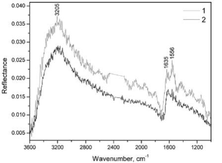
Figure 1: IR-RAS spectra of H₂O₂ solution just after pouring it in the cuvette. 1 (upper curve): the sample did not undergo the influence of the Teslar watch; 2 (lower curve): the sample was affected by the Teslar watch.

The behavior of a quantum system obeys the Schrödinger equation, which in our case can be written as follows

$$i{\kern 1.0pt}\hbar\frac{{\partial\psi\left({x,t}\right)}}{{\partial{\kern 1.0pt}t}}=-\frac{{\hbar^{2}}}{{2m}}\frac{{d^{2}\psi\left({x,t}\right)}}{{d{\kern 1.0pt}x^{2}}}+V\left({x,t}\right){\kern 1.0pt}{\kern 1.0pt}\psi\left({x,t}\right)$$ (65)

and the initial wave function $\psi\left({x,t}\right)$ is given as

$$\psi\left({x,{\kern 1.0pt}{\kern 1.0pt}{\kern 1.0pt}0}\right)=\left({2\pi\delta_{0}^{2}}\right)^{-0.25}{\kern 1.0pt}\exp\left[{i{\kern 0.5pt}p_{{\kern 0.5pt}0}{\kern 0.5pt}x/\hbar-\left({x-x_{0}}\right)^{2}/\left({2\delta_{0}}\right)^{2}}\right].$$ (66)

Here $x_{0}$, $\delta_{{\kern 0.5pt}0}$ and $p_{{\kern 0.5pt}0}$ are the initial position, width and momentum for the wave function of hydrogen atom, respectively. Figure 2 shows the base state of that hydrogen atom on O-H bonding.

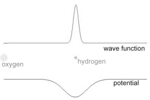
Figure 2: The base state of hydrogen atom on the O-H bonding.

Figure 3 shows the feature of the absolute value of wave function of that hydrogen atom after being irradiated by the infrared beam from FTIR.

The wave function of hydrogen atom vibrates right and left absorbing the infrared energy. However, when turning on the Teslar watch, the wave is broken in pieces and the vibration nearly stops due to the effect of inerton absorption as shown in Figure 4. The absorption of inertons can be modulated in quantum mechanics by introducing of the potential V in equation (65) in the form similar to the Newton’s one,

$$V\left({x,t}\right)=-\frac{\alpha}{x}{\kern 1.0pt}\cos\left({\Omega{\kern 1.0pt}{\kern 1.0pt}t}\right).$$ (67)

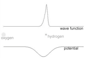
Figure 3: The wave function of the hydrogen atom changes under the IR from FTIR.

There have been the following choices and parameters that have been tuned in our simulator: 1) Rep. No. is the number of iterations of the discretized Schrödinger equation; 2) IR.p is the wave length of irradiated IR (the resonant wave length is around 300); I.pot is the amplitude of additional potential brought by inertons. It corresponds to the $\alpha$ in our equation with the multiplier: 50,000, for example, the 5,000 for I.pot is equivalent to 0.1 for $\alpha$; 3) I.delta is the coefficient that is used for modifying the additional term in our equation (65) as

$$\left({\alpha/x}\right)\times\cos\left({\Omega{\kern 1.0pt}t}\right)\Rightarrow\left({\alpha/\left({\rm x+I.delta}\right)\times\cos\left({\Omega{\kern 1.0pt}t}\right)}\right)$$

to avoid the singularity on $x=0$; 4) J.pot (off/on) allow us to consider the effect of another O-H bonding. If J.pot is on, the distance of these two O-H bonding is turned with the parameter “another .H”; 5) FTIR (off/on) allow us to treat whether FTIR is on or off.

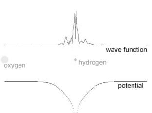
Figure 4: The wave is broken in pieces and the vibration nearly stops due to the effect of inerton absorption when turning on the Teslar watch.

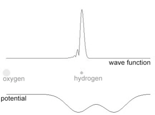
Figure 5: Hydrogen bonding between two water molecules.

As another possibility, we may try to simulate the effect of hydrogen bonding between two water molecules. This time the potential has two valleys caused from two different O-H bonding as shown in Figure 5. In this case the feature of vibration of hydrogen atom is almost the same as the case without considering the other O-H bonding shown in Figure 3. However when reducing the distance between two valleys, i.e. making closer two water molecules, the wave has broken in pieces and the vibration of wave function of hydrogen atom has ceased as shown in Figure 6. This means that O-H bonding no longer absorbs the energy from IR.

Thus the simulation of quantum mechanical problem by a classical scheme gives an information only on the behavior of $\psi$ function and does not clarify the reasons for the potential V that remains pure classical in non-deterministic quantum equation (65). The submicroscopic concept allows us to account for the origin of the potential V and gives a deeper analysis of the problem.

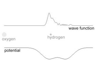
Figure 6: Two water molecules become closer; the wave function has broken in pieces and the vibration of wave function of hydrogen atom has ceased.

7. Concluding remarks

As many scientists who have dealt with thermodynamics, we have often had the impression that thermodynamics is easier to use than to understand. In such a situation, it is of real comfort to discover in books written by other scientists that they have felt the same impression. While two of these books only have been referenced herein, Refs. [3,4], we would like to express our gratitude to all the authors who have transmitted such a message, which is indubitably of great scientific interest.

In the present paper, by means of both conventional thermodynamic methods and the submicroscopic analysis, we have shown that the change in mass is a general law of evolution of physical systems. The mass exchange is the fundamental property of any physical system, from a system of several canonical particles to that of cosmological objects. Hitherto the defect of mass has being taken into account only in problems associated with nuclear physics. However, the present research points to the necessity of including the phenomenon of the defect of mass also in tasks typical for condensed matter physics. Besides, the submicroscopic consideration has allowed us to give an estimation of the speed of inertons, carriers of quantum mechanical and gravitational interactions of objects, which has been evaluated as about $2.5\times 10^{10}$ m/s.

Acknowledgement

We thank greatly Harry Yosh for the help in simulation.

References

- [1] E. Fermi, Thermodynamics (Prentice-Hall; New York, 1937).
- [2] P. Atkins and J. de Paula, Physical Chemistry, Seventh edition, (Oxford Universiry Press, 2002).
- [3] D. K. Nordstrom and J. L. Munoz, Geochemical thermodynamics (Blackwell Scientific Publications, 1986).
- [4] G. M. Anderson and D. A. Crerar, Thermodynamics in geochemistry (Oxford University Press, 1993).
- [5] J.-L. Tane, Evidence for a close link between the laws of thermodynamics and the Einstein mass-energy relation, J. Theoretics, June/July 2000, vol. 2 no. 3
- [6] J.-L. Tane, Thermodynamics, relativity and gravitation: evidence for a close link between the three theories, J. Theoretics, August/September 2001, vol. 3, no. 4
- [7] J.-L. Tane, Thermodynamics, relativity and gravitation in chemical reactions. A revised interpretation of the concepts of entropy and free energy, J. Theoretics 2002, extensive papers.
- [8] J.-L. Tane, Inert matter and living matter: a thermodynamic interpretation of their fundamental difference, J. Theoretics, June/July 2003, vol. 5, no. 3.
- [9] J.-L. Tane, Relativity, quantum mechanics, and classical physics, evidence for a close link between the three theories, J. Theoretics, Dec 2004, vol. 6, no. 6.
- [10] V. D. Zelepukhin, I. D. Zelepukhin and V. Krasnoholovets, Thermodynamic features and molecular organization of degassed aqueous system; English translation: Sov. Jnl. Chem. Phys. 12, 1461-84 (1994).
- [11] V. Krasnoholovets, P. Tomchuk and S. Lukyanets, Proton transfer and coherent phenomena in molecular structures with hydrogen bonds, Adv. Chem Phys. 125, ch. 5, 351-548 (2003).
- [12] M. Bounias and V. Krasnoholovets, Scanning the structure of ill-known spaces: Part 1. Founding principles about mathematical constitution of space, Kybernetes: The Int. J. Systems and Cybernetics, 32, 945-975 (2003) (also physics/0211096).
- [13] M. Bounias and V. Krasnoholovets, Scanning the structure of ill-known spaces: Part 2. Principles of construction of physical space, ibid. 32, 976-1004 (2003) (also physics/0212004).
- [14] M. Bounias and V. Krasnoholovets, Scanning the structure of ill-known spaces: Part 3. Distribution of topological structures at elementary and cosmic scales, ibid. 32, 1005-1020 (2003) (also physics/0301049).
- [15] V. Krasnoholovets and D. Ivanovsky, Motion of a particle and the vacuum, Phys. Essays 6, 554-563 (1993) (also quant-ph/9910023).
- [16] V. Krasnoholovets, Motion of a relativistic particle and the vacuum, Phys. Essays 10, 407-416 (1997) (also quant-ph/9903077).
- [17] V. Krasnoholovets. On the nature of spin, inertia and gravity of a moving canonical particle, Ind. J. Theor. Phys. 48, 97-132 (2000) (also quant-ph/0103110).
- [18] V. Krasnoholovets, Space structure and quantum mechanics, Spacetime & Substance 1, 172-175 (2000) (also quant-ph/0106106).
- [19] V. Krasnoholovets, Submicroscopic deterministic quantum mechanics, Int. J. Computing Anticipatory Systems 11, 164-179 (2002) (also quant-ph/0103110).
- [20] V. Krasnoholovets, Gravitation as deduced from submicroscopic quantum mechanics, also hep-th/0205196.
- [21] V. Krasnoholovets, On the mass of elementary carriers of gravitational interaction, Spacetime & Substance 2, 169-170 (2001) (also quant-ph/0201131).
- [22] V. Krasnoholovets, E. Andreev, G. Dovbeshko, S. Skliarenko and O. Strokach, The investigation of physical characteristics of the Teslar watch, Project funded by Teslar Inside Corporation, http://www.philipsteinteslar.com (has to be published).
- [23] G. Rein, Effect of Non-Hertzian waves on the immune system, JUS Psychotronics Association 1, 15-19 (1989).
- [24] G. Rein, Biological Interactions with Scalar Energy Cellular Mechanisms of Action, From The Proceedings 7th International Association of Psychotronics Research. Georgia. (Dec 1988).
- [25] A. S. Morley, The Teslar wrist watch, in: Health Consciousness 11, 44-46, June (1991).