Focusing and phase compensation of paraxial beams by a left-handed material slab

Abstract

On the basis of angular spectrum representation, a formalism describing paraxial beams propagating through an isotropic left-handed material (LHM) slab is presented. The treatment allows us to introduce the ideas of beam focusing and phase compensation by LHM slab. Because of the negative refractive index of LHM slab, the inverse Gouy phase shift and the negative Rayleigh length of paraxial Gaussian beam are proposed. It is shown that the phase difference caused by the Gouy phase shift in right-handed material (RHM) can be compensated by that caused by the inverse Gouy phase shift in LHM. If certain matching conditions are satisfied, the intensity and phase distributions at object plane can be completely reconstructed at the image plane.

I Introduction

In the late 1960s, Veselago firstly introduced the concept of left-handed material (LHM) in which both the permittivity $\varepsilon$ and the permeability $\mu$ are negative Veselago1968 . Veselago predicted that electromagnetic waves incident on a planar interface between a right-handed material (RHM) and a LHM will undergo negative refraction. Theoretically, a LHM planar slab can act as a lens and focus waves from a point source. Experimentally, the negative refraction has been observed by using periodic wires and rings structure Smith2000 ; Shelby2001 ; Pacheco2002 ; Parazzoli2003 ; Houck2003 . In the past few years, negative refractions in photonic crystals Notomi2000 ; Luo2002a ; Luo2002b ; Li2003 and anisotropic metamaterials Lindell2001 ; Hu2002 ; Smith2003 ; Zhang2003 ; Luo2005 have also been reported.

Recently, Pendry extended Veslago’s analysis and further predicted that a LHM slab can amplify evanescent waves and thus behaves like a perfect lens Pendry2000 . It is well known that in a conventional imaging system the evanescent waves are drastically decayed before they reach the image plane. While in a LHM slab system, both the phases of propagating waves and the amplitudes of evanescent waves from a near-field object could be restored at its image. Therefore, the spatial resolution of the superlens can overcome the diffraction limit of conventional imaging systems and reach the subwavelength scale. While great research interests were initiated by the revolutionary concept Smith2004a ; Smith2004b ; Parazzoli2004 ; Dumelow2005 , hot debates were also raised Hooft2001 ; Williams2001 ; Ziolkowski2001 ; Valanju2002 ; Garcia2002a ; Garcia2002b ; Vesperinas2004 .

The main purpose of the present work is to investigate the paraxial beams propagating through an isotropic LHM slab. Starting from the representation of plane-wave angular spectrum, we derive the propagation of paraxial beams in RHM and LHM. Our formalism permits us to introduce ideas for beam focusing and phase compensation of paraxial beams by using LHM slab. Because of the negative refractive index, the inverse Gouy phase shift and negative Rayleigh length in LHM slab are proposed. As an example, we obtain the analytical description for a Gaussian beam propagating through a LHM slab. We find that the phase difference caused by the Gouy phase shift in RHM can be compensated by that caused by the inverse Gouy phase shift in LHM.

II The Paraxial model of beam propagation

In this section, we present a brief derivation on paraxial model in RHM and LHM. Following the standard procedure, we consider a monochromatic electromagnetic field ${\bf E}({\bf r},t)=Re[{\bf E}({\bf r})\exp(-i\omega t)]$ and ${\bf B}({\bf r},t)=Re[{\bf B}({\bf r})\exp(-i\omega t)]$ of angular frequency $\omega$ propagating through an isotropic material. The field can be described by Maxwell’s equations Born1997

$$\nabla\times{\bf E} = -\frac{\partial{\bf B}}{\partial t},$$

$$\nabla\times{\bf H} = \frac{\partial{\bf D}}{\partial t},$$

$${\bf D} = \varepsilon{\bf E},$$

$${\bf B} = \mu{\bf H}.$$ (1)

One can easily find that the wave propagation is only permitted in the medium with $\varepsilon,\mu>0$ or $\varepsilon,\mu<0$. In the former case, ${\bf E}$, ${\bf H}$ and ${\bf k}$ form a right-handed triplet, while in the latter case, ${\bf E}$, ${\bf H}$ and ${\bf k}$ form a left-handed triplet. The previous Maxwell equations can be combined straightforwardly to obtain the well-known equation for the complex amplitude of the electric field in RHM or LHM

$$\nabla^{2}\ {\bf E}-\nabla(\nabla\cdot{\bf E})+k^{2}{\bf E}=0,$$ (2)

where $k=n_{R,L}\omega/c$, $c$ is the speed of light in vacuum, $n_{R}=\sqrt{\varepsilon_{R}\mu_{R}}$ and $n_{L}=-\sqrt{\varepsilon_{L}\mu_{L}}$ are the refractive index of RHM and LHM, respectively Veselago1968 .

Equation (2) can be conveniently solved by employing the Fourier transformations, so the complex amplitude in RHM and LHM can be conveniently expressed as

$${\bf E}({{\bf r}_{\bot}},z)=\int d^{2}{\bf k}_{\bot}\tilde{E}({\bf k}_{\bot})\exp[i{\bf k}_{\bot}\cdot{\bf r}_{\perp}+ik_{z}z].$$ (3)

Here ${\bf r}_{\perp}=x{\bf e}_{x}+y{\bf e}_{y}$, ${\bf k}_{\perp}=k_{x}{\bf e}_{x}+k_{y}{\bf e}_{y}$, and $e_{j}$ is the unit vector in the $j$-direction. Note that $k_{z}=\sigma\sqrt{n_{R,L}^{2}k^{2}_{0}-k^{2}_{\perp}}$, $\sigma=1$ for RHM and $\sigma=-1$ for LHM. The choice of sign ensures that power propagates away from the surface to the $+z$ direction. The field $\tilde{E}({\bf k}_{\bot})$ In Eq. (3) is related to the boundary distribution of the electric field by means of the relation

$$\tilde{{\bf E}}({\bf k}_{\bot})=\int d^{2}{\bf r}_{\bot}{\bf E}({\bf r}_{\bot},0)\exp[i{\bf k}_{\bot}\cdot{\bf r}_{\perp}],$$ (4)

which is a standard two-dimensional Fourier transform Goodman1996 . In fact, after the electric field on the plane $z=0$ is known, Eq. (3) together with Eq. (4) provides the expression of the field in the space $z>0$.

From a mathematical point of view, the approximate paraxial expression for the field can be obtained by the expansion of the square root of $k_{z}$ to the first order in $|{\bf k}_{\bot}|/k$ Lax1975 ; Ciattoni2000 , which yields

$${\bf E}({{\bf r}_{\bot}},z)= \exp(in_{R,L}k_{0}z)\int d^{2}{\bf k}_{\bot}$$ (5)

$$\times\exp\bigg{[}i{\bf k}_{\perp}\cdot{\bf r}_{\perp}-\frac{i{\bf k}_{\perp}z}{2n_{R,L}k_{0}}\bigg{]}\tilde{\bf E}({\bf k}_{\perp}).$$

Since our attention will be focused on beam propagating along the $+z$ direction, we can write

$${\bf E}({\bf r}_{\perp},z)={\bf A}({\bf r}_{\perp},z)\exp(in_{R,L}k_{0}z),$$ (6)

where the field $A({\bf r}_{\perp},z)$ is the slowly varying envelope amplitude which satisfies the parabolic equation

$$\bigg{[}i\frac{\partial}{\partial z}+\frac{1}{2n_{R,L}k_{0}}\nabla_{\perp}^{2}\bigg{]}{\bf A}({\bf r}_{\perp},z)=0,$$ (7)

where $\nabla_{\perp}=\partial_{x}{\bf e}_{x}+\partial_{y}{\bf e}_{y}$. From Eq. (7) we can find that the field of paraxial beams in LHM can be written in the similar way to that in RHM, while the sign of the refractive index is reverse.

III The propagation of paraxial Gaussian beam

The previous section outlined the paraxial model for general laser beams propagating in RHM and LHM. In this section we shall investigate the analytical description for a beam with a boundary Gaussian distribution. This example allows us to describe the new features of beam propagation in LHM slab. As shown in Fig. 1, the LHM slab in region $2$ is surrounded by the usual RHM in region $1$ and region $3$. The beam will pass the interfaces $z=a$ and $z=a+d$ before it reaches the image plane $z=a+b+d$. To be uniform throughout the following analysis, we introduce different coordinate transformations $z_{i}^{\ast}(i=1,2,3)$ in the three regions, respectively.

First we want to explore the field in region $1$. Without any loss of generality, we assume that the input waist locates at the object plane $z=0$. The fundamental Gaussian spectrum distribution can be written in the form

$${\bf E}_{1}({\bf k}_{\perp})=\frac{w_{0}}{\sqrt{2\pi}}\exp\bigg{[}-\frac{k_{\perp}^{2}w_{0}^{2}}{4}\bigg{]},$$ (8)

where $w_{0}$ is the spot size. By substituting Eq. (8) into Eq. (5), the field in the region $1$ can be written as

$${\bf E}_{1}({\bf r}_{\perp},z_{1}^{\ast})=\frac{w_{0}}{w_{1}(z_{1}^{\ast})}\exp\bigg{[}-\frac{r_{\perp}^{2}}{w_{1}^{2}(z_{1}^{\ast})}+i\psi_{1}(r_{\perp},z_{1}^{\ast})\bigg{]},$$ (9)

$$\psi_{1}(r_{\perp},z_{1}^{\ast}) = n_{R}k_{0}z_{1}^{\ast}+\frac{n_{R}k_{0}r_{\perp}^{2}}{2R_{1}(z_{1}^{\ast})}-\arctan\frac{z_{1}^{\ast}}{z_{R}},$$ (10)

$$w_{1}(z_{1}^{\ast}) = w_{0}\sqrt{1+(z_{1}^{\ast}/z_{R})^{2}},$$ (11)

$$R_{1}(z_{1}^{\ast}) = z_{1}^{\ast}+\frac{z_{R}^{2}}{z_{1}^{\ast}}.$$ (12)

Here $z_{1}^{\ast}=z$, $z_{R}=n_{R}k_{0}w_{0}^{2}/2$ is the Rayleigh length, $w_{1}(z_{1}^{\ast})$ is the beam size and $R_{1}(z_{1}^{\ast})$ the radius of curvature of the wave front. The first term and the second term in Eq. (10) are the plane wave phase and radial phase, respectively. The third term in Eq. (10) denotes the Gouy phase is given by $\Phi_{1}=-\arctan(z_{1}^{\ast}/z_{R})$.

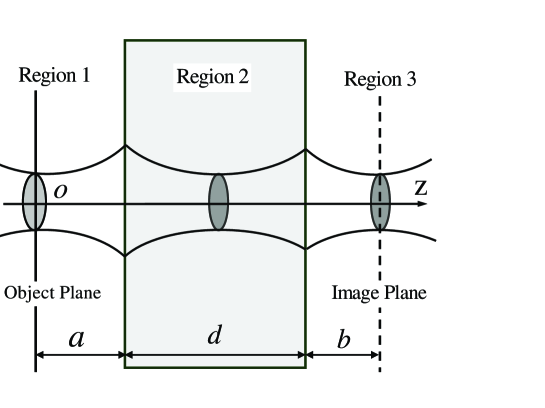
Figure 1: The mechanisms for paraxial beams propagating through an isotropic LHM slab. The LHM slab in region $2$ is surrounded by the usual RHM in region $1$ and region $3$. The solid line and the dashed line are the theoretical object and image planes, respectively.

We are now in a position to calculate the field in region $2$. In fact, the field in the first boundary can be easily obtained from Eq. (9) by choosing $z=a$. Substituting the field into Eq. (4), the angular spectrum distribution can be obtained as

$${\bf E}_{2}({\bf k}_{\perp})=\frac{w_{0}}{\sqrt{2\pi}}\exp\bigg{[}-\frac{k_{\perp}^{2}(n_{R}k_{0}w_{0}^{2}+2ia)}{4n_{R}k_{0}}\bigg{]},$$ (13)

For simplicity, we assume that the wave propagates through the boundary without reflection. Substituting Eq. (13) into Eq. (5), the field in the LHM slab can be written as

$${\bf E}_{2}({\bf r}_{\perp},z_{2}^{\ast})=\frac{w_{0}}{w_{2}(z_{2}^{\ast})}\exp\bigg{[}-\frac{r_{\perp}^{2}}{w_{2}^{2}(z_{2}^{\ast})}+i\psi_{2}(r_{\perp},z_{2}^{\ast})\bigg{]},$$ (14)

$$\psi_{2}(r_{\perp},z_{2}^{\ast}) = n_{L}k_{0}z_{2}^{\ast}+\frac{n_{L}k_{0}r_{\perp}^{2}}{2R_{2}(z_{2}^{\ast})}-\arctan\frac{z_{2}^{\ast}}{z_{L}},$$ (15)

$$w_{2}(z_{2}^{\ast}) = w_{0}\sqrt{1+(z_{2}^{\ast}/z_{L})^{2}},$$ (16)

$$R_{2}(z_{2}^{\ast}) = z_{2}^{\ast}+\frac{z_{L}^{2}}{z_{2}^{\ast}},$$ (17)

Here $z_{2}^{\ast}=z-(1-n_{L}/n_{R})a$ and $z_{L}=n_{L}k_{0}w_{0}^{2}/2$ is the Rayleigh length in LHM. The beam size $w_{2}(z_{2}^{\ast})$ and the radius of curvature $R_{2}(z_{2}^{\ast})$ are given by Eq. (16) and Eq. (17), respectively. The Gouy phase shift in LHM is given by $\Phi_{2}=-\arctan(z_{2}^{\ast}/z_{L})$.

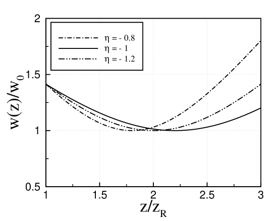
Figure 2: Plot of the beam widths in LHM slab with different refractive indices. The solid ($\eta=-1$), dash-dot-dotted ($\eta=-1.2$), and dash-dotted ($\eta=-0.8$) lines indicate the beam widths in LHM slab, where we assume $a=z_{R}$ and $\eta=n_{L}/n_{R}$. One can find the beams can be focused by LHM slab and the focusing waists remain $w_{0}$.

We note two interesting features of the paraxial field in LHM: First, because of the negative index of refraction, the inverse Gouy phase shift and negative Rayleigh length should be introduced. Second, the beams can be focused by LHM slab and the focusing waists remain $w_{0}$. For the purpose of illustration, the relevant focusing feature is shown in Fig. 2. We find that the place of focusing waist could be different which depends on the choice of the refractive index.

Finally we want to study the field in region $3$. The field in the second boundary can be easily obtained from Eq. (14) under choosing $z=a+d$. Substituting the field into Eq. (4), the angular spectrum distribution can be written as

$${\bf E}_{3}({\bf k}_{\perp})=\frac{w_{0}}{\sqrt{2\pi}}\exp\bigg{[}-\frac{k_{\perp}^{2}(n_{R}n_{L}k_{0}w_{0}^{2}+2in_{L}a+2in_{R}d)}{4n_{R}n_{L}k_{0}}\bigg{]}.$$ (18)

Substituting Eq. (18) into Eq. (5), the field in the LHM slab is given by

$${\bf E}_{3}({\bf r}_{\perp},z_{3}^{\ast})=\frac{w_{0}}{w_{3}(z_{3}^{\ast})}\exp\bigg{[}-\frac{r_{\perp}^{2}}{w_{3}^{2}(z_{3}^{\ast})}+i\psi_{3}(r_{\perp},z_{3}^{\ast})\bigg{]},$$ (19)

$$\psi_{3}(r_{\perp},z_{3}^{\ast}) = n_{R}k_{0}z_{3}^{\ast}+\frac{n_{R}k_{0}r_{\perp}^{2}}{2R_{3}(z_{3}^{\ast})}-\arctan\frac{z_{3}^{\ast}}{z_{R}},$$ (20)

$$w_{3}(z_{3}^{\ast}) = w_{0}\sqrt{1+(z_{3}^{\ast}/z_{R})^{2}},$$ (21)

$$R_{3}(z_{3}^{\ast}) = z_{3}^{\ast}+\frac{z_{R}^{2}}{z_{3}^{\ast}}.$$ (22)

Here $z_{3}^{\ast}=z-(1-n_{R}/n_{L})d$. The beam size $w_{3}(z_{3}^{\ast})$ and the radius of curvature $R_{3}(z_{3}^{\ast})$ are given by Eq. (21) and Eq. (22), respectively. The Gouy phase shift is given by $\Phi_{3}=-\arctan(z_{3}^{\ast}/z_{R})$.

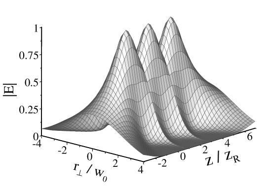
Figure 3: Numerically computed spatial map of the magnitude of the electric field for Gaussian beam propagating through the LHM slab. We assume $a=z_{R}$, $d=2z_{R}$ and $n_{L}=-n_{R}$. The first focusing waist in LHM slab locates at the plane $z/z_{R}=2$, while the second focusing waist in region $3$ locates at the plane $z/z_{R}=4$.

To this end, the fields are determined explicitly in the three regions. Comparing Eq. (14), Eq. (19) with Eq. (9) show that the field distributions in region $2$ and region $3$ still remain Gaussian. For the purpose of illustration, the spatial map of the electric fields is plotted in Fig. 3. We can easily find that there exists an internal and an external focus.

IV Beam focusing and phase compensation

In this section we examine the matching conditions of beam focusing and phase compensation. First we want to explore the matching condition of focusing. We can easily find the place of the focusing waist by choosing $z^{\ast}_{i}=0$. We assume the incident beam waist locates at plane $z=0$. After setting $z^{\ast}_{2}=0$ in Eq. (16), we get the first focusing waist in LHM slab locates at the plane $z=(1-n_{L}/n_{R})a$. Then we substitute $z^{\ast}_{3}=0$ into Eq. (16), we can find the second focusing waist in region $3$ locates at the plane $z=(1-n_{R}/n_{L})d$. We take the image position $z=a+d+b$ to be the place of the second focusing waist. Using this criterion, the matching condition for focusing can be written as

$$n_{L}(a+b)+n_{R}d=0.$$ (23)

In addition, the thickness of the LHM slab should satisfy the relation $d>-an_{L}/n_{R}$, otherwise there is neither an internal nor an external focus.

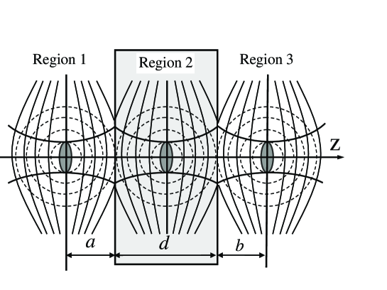
Figure 4: The phase difference caused by the Gouy phase shift in RHM can be compensated by that caused by the inverse Gouy phase shift in LHM slab. The phase fronts of Gaussian beam (solid lines) differ from those of a perfect spherical wave (dashed lines).

Next we attempt to investigate the matching condition for phase compensation. It is known that an electromagnetic beam propagating through a focus experiences an additional $\pi$ phase shift with respect to a plane wave. This phase anomaly was discovered by Gouy in 1890 and has since been referred to as the Gouy phase shift Siegman1986 ; Feng2001 . It should be mentioned that there exists an effect of accumulated Gouy phase shift when a beam passing through an optical system with positive index Erden1997 ; Feng1999 ; Feng2000 . While in the LHM slab system we expect that the phase difference caused by Gouy phase shift can be compensated by that caused by the inverse Gouy shift in LHM. In Fig. 4, we plot the distribution of phase fronts in the three regions. The phase difference caused by the Gouy phase shift in the three regions are given by

$$\Delta\Phi_{1} = -\arctan\frac{a}{z_{R}},$$

$$\Delta\Phi_{2} = -\arctan\frac{-n_{L}a}{n_{R}z_{L}}-\arctan\frac{-n_{L}b}{n_{R}z_{L}},$$

$$\Delta\Phi_{3} = -\arctan\frac{b}{z_{R}}.$$ (24)

The first and third Equations dictate the phase difference caused by the Gouy shift in region $1$ and region $3$, respectively. The second equation denotes the phase difference caused by the inverse Gouy phase shift in LHM slab. Subsequent calculations of Eq. (24) show

$$-\arctan\frac{a}{z_{R}}-\arctan\frac{b}{z_{R}}+\bigg{(}-\arctan\frac{-n_{L}a}{n_{R}z_{L}}-\arctan\frac{-n_{L}b}{n_{R}z_{L}}\bigg{)}=0.$$ (25)

This means that the phase difference caused by the Gouy phase shift in RHM can be compensated by that caused by the inverse Gouy phase shift in LHM slab. Therefore the condition for phase compensation can be simply written as

$$n_{R}k_{0}a+n_{R}k_{0}b+n_{L}k_{0}d=0.$$ (26)

The first two terms in Eq. (26) are the phase deference caused by the plane wave in RHM. The last term in Eq. (26) is the phase deference caused by the plane wave in LHM slab.

Finally we discuss the phase difference caused by the radial phase. Following the method outlined by Dumelow et al. Dumelow2005 , we assume that the beam waist locates at the object plane. Then we take the image position to be that where the intensity is a maximum. Evidently, from Eqs. (19)-(22) we can find that the intensity maximum locates at the plane of beam waist. The phase difference between the object plane and the image plane is independent of radial position, since the phase fronts are flat there.

The new message in this paper is to prove that the intensity and phase distributions at object plane can be completely reconstructed at the image plane by LHM slab. Now an interesting question naturally arises: whether the matching conditions of focusing and the phase compensation can be satisfied simultaneously. From Eqs. (23)-(26) one can easily find that the refractive index, $a$, $b$ and $d$ should satisfy the matching conditions:

$$n_{L}=-n_{R},~{}~{}~{}a+b=d.$$ (27)

Under the matching conditions, the reflected waves at the interface between RHM and LHM are completely absent. Therefore the intensity and phase distributions at the object plane can be completely reconstructed at the image plane.

Note that the purpose of this paper is to examine beam focusing and phase compensation in paraxial regime. The evanescent waves which are claimed to provide the subwavelength imaging do not correspond to the problem under study. The paraxial model only deals with beams whose transverse dimension is much larger than a wavelength. However, in the subwavelength focusing regime a rigorous diffraction theory should be developed.

V Conclusions

In conclusion, we have investigated the focusing and phase compensation of paraxial beams by an isotropic LHM slab. We have introduced the concepts of inverse Gouy phase shift and negative Rayleigh length of paraxial beams in LHM. We have shown that the phase difference caused by the Gouy phase shift in RHM can be compensated by that caused by the inverse Gouy phase shift in LHM slab. If certain matching conditions are satisfied, the intensity and phase distributions at object plane can be completely reconstructed at the image plane. We expect many potential devices can be constructed based on the paraxial beam model discussed above. They can, for example, be used to provide beam focusing, phase compensation and image transfer.

- (1) V.G. Veselago, Sov. Phys. Usp. 10 (1968) 509.
- (2) D.R. Smith, W.J. Padilla, D.C. Vier, S.C. Nemat-Nasser, S. Schultz, Phys. Rev. Lett. 84 (2000) 4184.
- (3) R.A. Shelby, D.R. Smith, S. Schultz, Science 292 (2001) 77.
- (4) J. Pacheco Jr., T.M. Grzegorczyk, B.I. Wu, Y. Zhang, J.A. Kong, Phys. Rev. Lett. 89 (2002) 257401.
- (5) C.G. Parazzoli, R.G. Greegpr, K. Li, B.E.C. Koltenba, M. Tanielian, Phys. Rev. Lett. 90 (2003) 107401.
- (6) A.A. Houck, J.B. Brock, I.L. Chuang, Phys. Rev. Lett. 90 (2003) 137401.
- (7) M. Notomi, Phys. Rev. B62 (2000) 10696.
- (8) C. Luo, S.G. Johnson, J.D. Joannopoulos, J.B. Pendry, Phys. Rev. B65 (2002) 201104.
- (9) C. Luo, S.G. Johnson, J.D. Joannopoulos, Appl. Phys. Lett. 81 (2002) 2352.
- (10) J. Li, L. Zhou, C.T. Chan, P. Sheng, Phys. Rev. Lett. 90 (2003) 083901.
- (11) I.V. Lindell, S.A. Tretyakov, K.I. Nikoskinen, S. Ilvonen, Microw. Opt. Technol. Lett. 31 (2001) 129.
- (12) L.B. Hu, S.T. Chui, Phys. Rev. B66 (2002) 085108.
- (13) D.R. Smith, D. Schurig, Phys. Rev. Lett. 90 (2003) 077405.
- (14) Y. Zhang, B. Fluegel, A. Mascarenhas, Phys. Rev. Lett. 91 (2003)157401.
- (15) H. Luo, W. Hu, X. Yi, H. Liu, J. Zhu, Opt. Commun. 254 (2005) 353.
- (16) J.B. Pendry, Phys. Rev. Lett. 85 (2000) 3966.
- (17) D.R. Smith, D. Schurig, J.J. Mock, P. Kolinko, P. Rye, Appl. Phys. Lett. 84 (2004) 2244 .
- (18) D.R. Smith, P. Kolinkp, D. Schurig, J. Opt. Soc. Am. B21 (2004) 1032.
- (19) C.G. Parazzoli, R.B. Greegor, J.A. Nielsen, M.A. Thompson, K. Li, A.M. Vetter, D.C. Vier Appl. Phys. Lett. 84 (2004) 3232.
- (20) T. Dumelow, J.A.P. da Costa, V.N. Freire, Phys. Rev. B72 (2005) 235115.
- (21) G.W.’t Hooft, Phys. Rev. Lett. 87 (2001) 249701.
- (22) J.M. Williams, Phys. Rev. Lett. 87 (2001) 249703.
- (23) R.W. Ziolkowski, E. Heyman, Phys. Rev. E64 (2001) 056625.
- (24) P.M. Valanju, R.M. Walser, A.P. Valanju, Phys. Rev. Lett. 88 (2002)187401.
- (25) N. Garcia, M. Nieto-Vesperinas, Opt. Lett. 27 (2002) 885.
- (26) N. Garcia, M. Nieto-Vesperinas, Phys. Rev. Lett. 88 (2002) 207403.
- (27) M. Nieto-Vesperinas, J. Opt. Soc. Am. A21 (2004) 491.
- (28) M. Born, E. Wolf, Principles of Optics, University Press, Cambridge, 1997.
- (29) J.W. Goodman, Introduction to Fourier Optics, McGraw-Hill, New York, 1996.
- (30) M. Lax, W.H. Louisell, W. McKnight, Phys. Rev. A11 (1975) 1365.
- (31) A. Ciattoni, B. Crosignani, P. Di Porto, Opt. Commun. 177 (2000) 9.
- (32) A.E. Siegman, Lasers, University Science, Mill Valley, 1986.
- (33) S. Feng, H.G. Winful, Opt. Lett. 26 (2001) 485.
- (34) M.F. Erden, H.M. Ozaktas, J. Opt. Soc. Am. A14 (1997) 2190.
- (35) S. Feng, H.G. Winful, J. Opt. Soc. Am. A16 (1999) 2500.
- (36) S. Feng, H.G. Winful, Phys. Rev. E61 (2000) 862.