Modelling and Simulations of Multi-component Lipid Membranes and Open Membranes via Diffusive Interface Approaches

Abstract

In this paper, phase field models are developed for multi-component vesicle membranes with different lipid compositions and membranes with free boundary. These models are used to simulate the deformation of membranes under the elastic bending energy and the line tension energy with prescribed volume and surface area constraints. By comparing our numerical simulations with recent experiments, it is demonstrated that the phase field models can capture the rich phenomena associated with the membrane transformation, thus it offers great functionality in the simulation and modeling of multicomponent membranes.

1 Introduction

Lipid vesicle membranes are ubiquitous in biological systems. Studies of vesicle self assembly and shape transition, including bud formation [24, 25, 31] and vesicle fission [13] are very important in the understanding of cell functions. In recent experimental studies, multi-component vesicles with different lipid molecule compositions (and thus phases) have been shown to display even more complex morphology involving rafts and micro-domains [2]. There are strong evidences suggesting that phase segregation and interaction contribute critically to the membrane signaling, trafficking and sorting processes [3]. In the literature, the geometric and topological structures of multi-component vesicles have been theoretically modeled by minimizing an energy with contributions of the bending resistance, that is the elastic bending energy, and the line tension at the interface between different components or the phase boundary [4, 20, 23, 26]. The elastic bending energy first studied by Canham, Evans and Helfrich [11, 12, 28] for a single-phase membrane is defined as

$$E=\int_{\Gamma}\left(a_{1}+a_{2}(H-c_{0})^{2}+a_{3}G\right)\,ds,$$ (1)

where $H$ is the mean curvature of the membrane surface $\Gamma$, $c_{0}$ the spontaneous curvature, $G$ the Gaussian curvature, $a_{1}$ the surface tension, $a_{2}$ the bending rigidity and $a_{3}$ the stretching rigidity.

In recent experimental studies, it has been found that the bending rigidity in the liquid-disordered phase differs from that in the liquid-ordered phase in two-component membranes [2, 3]. This can be attributed to, among other things, that the two phases have different lipid compositions or different concentrations of cholesterol molecules which serve as spacers between lipids. Thus, in the generalized bending elasticity model for two-component membranes, the bending rigidity $a_{2}$ is assumed to take values $k_{1}$ and $k_{2}$ respectively in two different components (phases) $\Gamma_{1}\subset\Gamma$ and $\Gamma_{2}\subset\Gamma$ (with $\Gamma=\Gamma_{1}\cup\Gamma_{2}$). The common phase boundary between the two phases is denoted by $\gamma_{0}=\Gamma_{1}\cap\Gamma_{2}$. In general, the other parameters may also vary in different phases, however, in this paper, we ignore the effect due to $a_{1},a_{3}$ and $c_{0}$ and concentrate only on the effect of the bending rigidity, though the methodology can be easily extended to more general case. In fact, the formulation we present here works for two components having possibly different spontaneous curvatures, but for simplicity such curvatures are set to be zero in the numerical simulations.

With the two phases co-existing on the membrane, it is natural to introduce a line tension on $\gamma_{0}$ to take into account the interfacial energy between the individual components [2, 22, 31]. Coupling with the bending elastic energy, this leads to the following total energy determining the two component membrane

$$E=E_{1}+E_{2}+E_{l}=\sum_{i=1}^{2}\int_{\Gamma_{i}}k_{i}(H-c_{i})^{2}\,ds+\int_{\gamma_{0}}\delta\,dl\;,$$ (2)

where $\delta$ is the line tension constant [22]. Note that in general, the line energy can also include the integral of a multiple of the curvature square on $\gamma_{0}$ [3].

The mathematical model that our study is based on is the minimization of the total energy defined in (2) for a two component membrane with a prescribed total volume, and prescribed surface areas of both components. In order to effectively model and simulate the experimental findings on the exotic morphology of the multi-component vesicles (mostly taken from [2]), we extend the recently developed phase field approach for the single component vesicles [18] to the multi-component case, which avoids the tracking of the vesicle membrane by viewing the surface and phase boundary as the zero level sets of phase field functions. The general phase field framework has been used successfully in many applications [1, 6, 9, 10]. For membrane deformation, this approach has become increasing popular in the research community in recent years. So far, its applications have mostly confined to the case of using a single phase field function [5, 15, 16, 21, 27], albeit it is known that co-dimension two objects can be described effectively by a pair of level-set or phase field functions [7, 10, 29, 32]. With the introduction of a second phase field function, we demonstrate that the new two-component phase field model is capable of capturing rich complex morphological changes experimentally observed in the two-component vesicle membranes. Moreover, this model can be very easily generalized to study the open membranes or membranes with free boundary (see [30] for experimental study and [8, 33, 34, 35, 37] for analysis and computation). This is based on the observation that an open membrane can be thought as a two component vesicles with one component having zero bending rigidity. Further generalization is possible for vesicles with three or more components.

The paper is organized as follows: in section 2, we present the phase field formulation of the total energy (2) and address the approach of penalty formulation for the constraints. In section 3, we first briefly discuss the discretization schemes and some implementation issue. After presenting some convergence tests to validate our method, we assemble a number of interesting experiments to explore the shape transformations due to the changes of different parameters. The numerical simulations are compared with experimental findings including the merge and splitting of different components. In section 5, we present the phase field formulation for open membranes and some numerical simulation results. We then make some conclusion remarks in section 6. Some technical derivations are provided in the appendix.

2 A diffusive interface model

We start by introducing a pair of phase field functions $(\phi({\bf x}),\eta({\bf x}))$, defined on the physical (computational) domain $\Omega$.

The function $\phi=\phi({\bf x})$ is used so that the level set $\{{\bf x}:\phi{({\bf x})}=0\}$ gives the membrane $\Gamma$, while $\{{\bf x}:\phi{({\bf x})}>0\}$ represents the interior of the membrane (denoted by $\Omega_{i}$) and $\{{\bf x}:\phi{({\bf x})}<0\}$ the exterior (denoted by $\Omega_{e}$). In the phase field models of a single component vesicle, this is the only phase field function used [17].

Next, we take another closed surface $\Gamma_{\bot}$ defined on domain $\Omega$ and being perpendicular to $\Gamma$, such that it is the zero level set $\{{\bf x}:\eta{({\bf x})}=0\}$ of a phase field function $\eta=\eta(x)$ in $\Omega$ with $\{{\bf x}:\eta{({\bf x})}>0\}$ being the interior of $\Gamma_{\bot}$ and $\{{\bf x}:\phi{({\bf x})}<0\}$ the exterior. We thus take the part of $\Gamma$ in the interior of $\Gamma_{\bot}$ as the first component $\Gamma_{1}$ and the remain part of $\Gamma$ (denoted by $\Gamma_{2}$) makes up the second component. Note that there may be many choices to select $\Gamma_{\bot}$, but we are mostly interested in the level set $\{{\bf x}:\eta{({\bf x})}=\phi{({\bf x})}=0\}$ which gives the boundary between two components, with $\{{\bf x}:\eta{({\bf x})}>0\mbox{ and }\phi({\bf x})=0\}$ representing one component of the membrane and $\{{\bf x}:\eta{({\bf x})}<0\mbox{ and }\phi({\bf x})=0\}$ the other component.

In the phase field modelling, the functions $\eta$ and $\phi$ are forced to be nearly constant valued except in thin regions near the surfaces $\Gamma$ and $\Gamma_{\bot}$ respectively. We use two small positive constant parameters $\epsilon$ and $\xi$ to characterize the widths of the thin regions (also called the diffusive interfaces). We note that a phase field function (order parameter), like our $\eta$, has been introduced in [21, 27] to describe the phase segregation on the membranes, but different from our phase field description of the surface $\Gamma$, an explicit construction of the membrane surface and a direct computation of the bending elastic energy are used there instead of the phase field representation of the membrane surface.

Similar to [15], we have the phase field elastic bending energy defined by

$$E(\phi,\eta)=\int_{\Omega}\frac{k(\eta)}{2\epsilon}\big{(}\epsilon\Delta\phi+(\frac{1}{\epsilon}\phi+c_{0}(\eta)\sqrt{2})(1-\phi^{2})\big{)}^{2}\,dx,$$ (3)

where we take a variable bending rigidity given by $k(\eta)=k+c\tanh(\frac{\eta}{\xi})$, so that $k+c$ corresponds to the value of the bending rigidity of one component and $k-c$ the other. Similarly, $2c_{0}(\eta)=(c_{1}+c_{2})+(c_{1}-c_{2})\tanh(\frac{\eta}{\xi})$, so that $c_{1}$ and $c_{2}$ correspond to the spontanenous curvatures in the two components respectively. A few other functionals needed in our model are as follows:

$$L(\phi,\eta)=\int_{\Omega}\delta[\frac{\xi}{2}|\nabla\eta|^{2}+\frac{1}{4\xi}(\eta^{2}-1)^{2}][\frac{\epsilon}{2}|\nabla\phi|^{2}+\frac{1}{4\epsilon}(\phi^{2}-1)^{2}]\,dx,$$ (4)

$$A(\phi)=\int_{\Omega}[\frac{\epsilon}{2}|\nabla\phi|^{2}+\frac{1}{4\epsilon}(\phi^{2}-1)^{2}]\,dx,$$ (5)

$$A(\phi)=\int_{\Omega}\phi\,dx,$$ (6)

$$D(\phi,\eta)=\int_{\Omega}\tanh(\frac{\eta}{\xi})[\frac{\epsilon}{2}|\nabla\phi|^{2}+\frac{1}{4\epsilon}(\phi^{2}-1)^{2}]\,dx\;.$$ (7)

To reveal the meaning of the above functionals, we follow similar discussions in [15] to assume an ansatz of the form $\phi({\bf x})\sim\tanh(d({\bf x},\Gamma)/(\sqrt{2}\epsilon))$ and $\eta({\bf x})\sim\tanh(d({\bf x},\Gamma_{\bot})/(\sqrt{2}\xi))$ for the phase field functions. Here $d$ denotes the signed distance function. In this ansatz, we can check that as $\epsilon$ and $\xi$ tend to $0$, that is, in the sharp interface limit,

$$E(\phi,\eta)\to\frac{2\sqrt{2}}{3}\sum_{i}\int_{\Gamma_{i}}k_{i}(H-c_{i})^{2}\,ds\;.$$ (8)

More details are given in the appendix, along with a brief derivation of the folllowing asymptotic limits

$$V(\phi)\to 2|\Omega_{i}|-|\Omega|\;,\quad A(\phi)\to\frac{2\sqrt{2}}{3}|\Gamma|\;,$$ (9)

and

$$L(\phi,\eta)\to\frac{8}{9}\int_{\gamma_{0}}\delta dl\;,\qquad D(\phi,\eta)\to\frac{2\sqrt{2}}{3}(|\Gamma_{1}|-|\Gamma_{2}|)\;.$$ (10)

To re-cap the discussion, the total energy in the phase field two-component model is

$${\cal E}(\phi,\eta)=E(\phi,\eta)+L(\phi,\eta)\;,$$ (11)

while the constraints are given by

$$V(\phi)=v_{d},\quad A(\phi)=a_{0},\quad D(\phi,\eta)=a_{d},$$ (12)

with $v_{d}$, $a_{t}$ and $a_{d}$ being the prescribed volume difference (hence the interior volume is prescribed), the total surface area and the area difference between the two components (hence areas of both components are prescribed).

To maintain the consistency of the phase field model which is based on $\phi$ and $\eta$ having the tanh profiles and the orthogonality between $\Gamma$ and $\Gamma_{\bot}$, additional constraints are imposed. First of all, the orthogonality constraint on the normal directions of the two surfaces, written in our phase field formulations, can be enforced by $\nabla\phi\cdot\nabla\eta=0$ on or near the phase boundary $\{{\bf x}:\phi({\bf x})=\eta({\bf x})=0\}$. With $\phi$ and $\eta$ having tanh profiles, their gradients become small away from their zero level sets, the orthogonality constraint may thus be enforced everywhere by penalizing

$$N(\phi,\eta)=\int_{\Omega}\frac{\epsilon}{2}|\nabla\phi\cdot\nabla\eta|^{2}\,dx\;.$$ (13)

Secondly, to better maintain the tanh profile of $\eta$, especially for the case with a large line tension energy, we have two options, one is to add a small regularization term, much like the bending elastic energy for $\phi$ but with a very small bending rigidity; another option is to regularize through the following functional

$$P(\eta)=\int_{\Omega}\big{(}\frac{\xi}{2}|\nabla\eta|^{2}-\frac{1}{4\xi}(\eta^{2}-1)^{2}\big{)}^{2}\,dx\;,$$ (14)

which also vanishes for any function $\eta$ with a tanh profile.

Summarizing the above, the variational phase field model to describe the two-component vesicles in the energy minimizing state is to minimize the total energy ${\cal E}(\phi,\eta)=E(\phi,\eta)+L(\phi,\eta)$ with constraints $V(\phi)=\alpha_{1}$, $A(\phi)=\alpha_{2}$, $D(\phi,\eta)=\alpha_{3}$ while $N(\phi,\eta)$ and $P(\eta)$ remain small. So, by adding both the penalty and regularization terms, the vesicle surface and the two components phase boundary are determined by a pair of phase functions $(\phi,\eta)$ which minimizes the energy

$$\ {\cal E}_{M}(\phi,\eta) = E(\phi,\eta)+L(\phi,\eta)+\frac{1}{2}M_{1}(V(\phi)-v_{d})^{2}+\frac{1}{2}M_{2}(A(\phi)-a_{0})^{2}$$ (15)

$$+\frac{1}{2}M_{3}(D(\phi,\eta)-a_{d})^{2}+\frac{1}{2}M_{4}(N(\phi,\eta))^{2}+\frac{1}{2}M_{5}(P(\eta))^{2}$$

where $\{M_{i}\}_{i=1}^{3}$ are penalty constants for the constraints on the volume and surface areas while $\{M_{i}\}_{i=4}^{5}$ are regularization constants for maintaining better control on the phase field functions.

3 Numerical Simulations of Two-Component Membranes

In this section, we compute the minimum of the phase field energy (15) by adopting a gradient flow approach which has been very effective for solving the phase field model of single component vesicles [17, 19]. The equations for the gradient flow are given by:

$$\phi_{t}=-\frac{\delta{\cal E}_{M}}{\delta\phi},\quad\eta_{t}=-\frac{\delta{\cal E}_{M}}{\delta\eta}\;.$$ (16)

The monotone decreasing of the energy $E_{M}$ is ensured for $t>0$. For simplicity, we only consider the case where $c_{1}=c_{2}=0$, this allows us to focus on examining how the variation in the bending rigidity alone affects the vesicle shape deformation and the equilibrium configurations of two-component membranes. The more general cases involving the spontaneous curvatures are to be considered in the future.

Discretization and code development.

We take the spatial computational domain as the box $\Omega=[-\pi,\pi]^{3}$ and assume that membranes are enclosed in the box. Moreover, we choose to set $\xi=\epsilon$ in our numerical simulations. For the spatial discretization of (16) in $\Omega$, a Fourier spectral method is used. Due to the regularization effect of the finite transition layer, for fixed $\epsilon$ and enough Fourier modes, the spectral method is an efficient way to solve (16) with the help of FFT routines [10]. A couple of options are implemented for the time discretization, such as an explicit forward Euler scheme or a semi-implicit Euler scheme [17]. The time step $\Delta t$ is chosen to ensure the energy decay. For most of our numerical experiments, although fully adjustable, $\Delta t$ is kept in the range of $10^{-6}$ to $10^{-7}$. The simulation codes are fully parallelized on both distributed memory systems via MPI and shared memory systems via OPENMP to improve its efficiency and functionality in conducting extensive three dimensional simulations.

Problem set up and initial profiles.

We now discuss how we choose various parameters in the simulations. Though in theory the gradient flow can be started from any pair of initial phase field functions, a proper choice often speeds up the evolution process and allows more efficient solution of the equilibrium state. With the penalty formulation, a particular constraint can be simply removed by setting the corresponding penalty constant zero. For example, setting $M_{2}=M_{3}=0$ would eliminate the total area and area difference constraints. This fact can be utilized to find good initial phase field functions.

For example, as illustrated in Figure.1, for a given $r>0$, we may start from two special phase field functions as $\phi({\bf x})=\tanh(\frac{|x|-r}{\sqrt{2}\epsilon})$ and $\eta({\bf x})=\tanh(\frac{z}{\sqrt{2}\epsilon})$ where $z$ is the third component of ${\bf x}$. This provides two hemispheres that represent the two components (colored in $red$ and $blue$ respectively, or in gray-scale represented by lighter and darker regions). Starting from this initial state, and setting $M_{1}=0$ to eliminate the volume constraint, the sphere gradually becomes more elliptical due to the presence of line tension, then further transform to a gourd like shape. We may stop at an intermediate shape and add back the volume constraint. This would provide a variety of initial shapes to be used in the simulations.

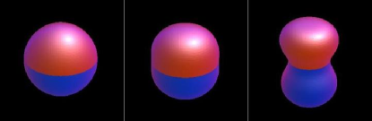
Fig. 1: Line tension drives a two-component sphere to a gourd shape.

Convergence verification.

For a particular numerical simulation, the quality of the numerical result may be affected by the choice of computational domain, the parameter $\epsilon$ (the effective width of the diffusive interface), the number of grid points, and the choices of other parameters used in the simulation. The parameter $\epsilon$ is generally taken to be a few percentage points of the domain size to ensure a relatively sharp interfacial region and the consistency with the sharp interface description (the $\epsilon\to 0$ limit). The mesh size is normally taken to be several times smaller than the width of the transition layer to ensure adequate spatial resolution. To ascertain the accuracy and robustness of our numerical algorithms and the parameter selections, we here present results of some numerical tests on the convergence and performance of our method.

The first set of experiments given in Figure 2 is designed to test the dependence of the resolution of the phase field function on the the parameter $\epsilon$ and grid size. We take a shape similar to the previous experiment. First, we take a $64^{3}$ grid but use different values of $\epsilon$ at $0.1964(=2h)$ and $0.1472(=1.5h)$. The other parameters are defined by $v_{d}=-216.52$, $a_{0}=29.46$, $a_{d}=0.23$ and $M_{i}=3.2\times 10^{5}$ for all $i$. The two equilibrium shapes are almost the same except the transition layer width. The corresponding final energy values $124.49$ and $123.82$ are very closed to each other. The left picture of Figure 2 gives the final three dimensional views and some cross section views of the phase field functions $\phi$ and $\eta$.

   

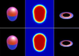
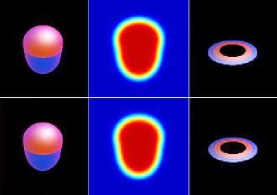
Fig. 2: The 3d and cross-section views of $\phi$ and the 3d view for part of $\eta$, computed with different parameters: left picture, $\epsilon=2h$ (above) and $\epsilon=1.5h$ (below); right picture, $64^{3}$ grid (above) and $48^{3}$ grid (below).

Now we use the same set of parameters ($\epsilon=0.1964$, same initial $\phi_{0}$ in the same domain), but solve the problem on two different grid sizes $48^{3}$ and $64^{3}$. We set the parameters $v_{d}=-216.52$, $a_{0}=29.46$, $a_{d}=0.23$ and constants $M_{i}=10^{4}$ for all $i$. The right picture of Figure 2 provides the details of the simulations, with the 3d views of $\phi$ and their density plots of the cross-sections in $x-z$ plan. The plots of the corresponding $\eta$ are similar to that in the third column of the left picture of Figure 2 and are thus omitted. The final values of energy are $124.39$ and $124.42$ while the elastic bending energy values are at $48.05$ and $47.96$, and the line tension energy values at $76.34$ and $76.46$ respectively. The close values substantiate the convergence of the simulated results.

The convergence can also be verified for different penalty and regularization constants $\{M_{i}\}_{i=1}^{5}$. The difference in the penalty and regularization is to be understood as follows: the penalty constants $\{M_{i}\}_{i=1}^{3}$ are taken to be larger and larger to ascertain the satisfaction of the volume and areas constraints. The regularization constants $\{M_{4},M_{5}\}$, on the other hand, are taken to be smaller and smaller so that while the orthogonality of the zero level sets of the two phase field functions and the tanh like profile of $\eta$ are both effectively maintained in the simulations, the associated energy contributions from the regularization terms in fact diminish.

First, we define the Lagrange multipliers by $\lambda_{i}=\lim_{M_{i}\rightarrow\infty}\Lambda_{i}(\{M_{i}\}_{1}^{3})$ with $\Lambda_{1}=M_{1}(V(\phi)-v_{d})$, $\Lambda_{2}=M_{2}(A(\phi)-a_{0})$, $\Lambda_{3}=M_{3}(D(\phi,\eta)-a_{d})$. With other parameters given ($M_{4}=M_{5}=10000$, $v_{d}=-216.52$, $a_{0}=29.46$, $a_{d}=0.230$, $\epsilon=1.768$, $h=0.17355$), we set larger and larger values for $M_{1}=M_{2}=M_{3}$. The results are given in Table 1 which show that $\Lambda_{1}$, $\Lambda_{2}$ and $\Lambda_{3}$ converge to the Lagrange multipliers, and errors in constraints also decrease.

$M_{1}=M_{2}=M_{3}$	4000	8000	16000	32000
$\Lambda_{1}$	-3.0781	-3.0823	-3.0946	-3.0943
$V(\phi)-v_{d}$ $(\times 10^{-4})$	-7.6952	-3.8528	-1.9341	-0.9669
$\Lambda_{2}$	3.6342	3.6430	3.6608	3.6626
$A(\phi)-a_{0}$ $(\times 10^{-4})$	9.0855	4.5537	2.2880	1.1445
$\Lambda_{3}$	0.8144	0.8144	0.8181	0.8173
$D(\phi,\eta)-a_{d}$ $(\times 10^{-4})$	2.0360	1.0180	0.5113	0.2554

Table 1: Convergence of the Lagrange multipliers.

Next, we demonstrate that the regularization terms provide effective control on the phase field functions but do not contribute significantly to the energy minimization. We set a sequence of decreasing values for $M_{4},M_{5}$ while taking the same values for $M_{1}=M_{2}=M_{3}=10000$, and keeping the values of other parameters the same as in the previous test. The results are given in Table 2 where $E_{4}=\frac{1}{2}M_{4}(N(\phi,\eta))^{2}$ and $E_{5}=\frac{1}{2}M_{5}(P(\eta))^{2}$ and their ratios with the total energy ${\cal E}_{M}$ are provided. We can observe the diminishing and negligible effect of the regularization terms while there is no noticeable change in the simulated membrane.

$M_{4}=M_{5}$ $(\times 10^{3})$	32	16	8	4
$E_{4}$	0.1223	0.1108	0.0966	0.0798
$E_{4}/{\cal E}_{M}$	0.0983%	0.0892%	0.0778%	0.0643%
$E_{5}$	0.0380	0.0336	0.0285	0.0227
$E_{5}/{\cal E}_{M}$	0.0305%	0.0270%	0.0229%	0.0182%
${\cal E}_{M}$	124.2942	124.2027	124.1209	124.0500

Table 2: The diminishing effect of regularization on the total energy.

Having demonstrated the convergence of the numerical algorithms, we next study the effect of different bending rigidities and various line tension constants. Then by adjusting the bending rigidities in the two components and the line tension, we can simulate the the vesicle shapes in experiment findings [2]. Unless noted otherwise, the simulation results reported in the following are obtained with a $64^{3}$ grid sizes and $\epsilon=0.1736$ which can provide sufficient resolution based on the convergence study.

Effect of the bending rigidities.

The values of bending rigidities often play a key role in forming various shapes of vesicles. Our first experiment is a simulation of the striped vesicles. We start from an initial shape where the red component is situated in the center to give a stripe-looking vesicle. As shown in the first row of the Figure 3, with parameters $v_{d}=-213.98$, $a_{0}=29.46$ and $a_{d}=-13.31$, the initial shape grows into a very regular stripe-looking ellipsoid shown in the middle of the first row. In this experiment, the bending rigidity for the red component is $1.0$ whereas the blue component is $3.0$. With line tension being fixed at $10.0$, we then make a switch of the bending rigidity of the two components. As shown in the right picture of the first row, the red component of the ellipsoid in the middle grows to a more cylindrical like shape. Next, by preserving the bending rigidity of the blue component while increasing that of the red component from $3.0$ to $19.0$, the red component shrinks in the middle and we get a thinner center band as shown in the left picture of the second row. It is obvious that the concave region has a smaller mean curvature. We can further increase the area of the blue component by setting $a_{0}=33.46$ and $a_{d}=-19.82$, and with bending rigidities $3.8$ and $0.2$ respectively for the red and blue components, we get the middle picture of the second row in Figure 3. One can compare it with the last picture found in actual experiments [2] though the differences of the bending rigidities are not as significant as those used here. In the final shape, the center band has the lowest mean curvature and it is occupied by the red component (having larger bending rigidities).

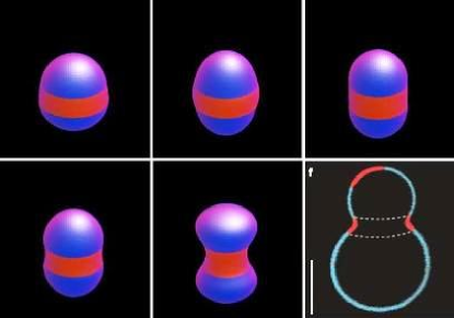
Fig. 3: Different values of bending rigidity lead to different shapes of striped vesicles (the right bottom picture is reproduced from [2]).

As expected, the numerical simulation shows that the component with a larger bending rigidity is more likely to remain in regions with smaller values of mean curvature.

Effect of line tension constants.

By intuition, we expect that larger line tension generally leads to a shorter interfacial line between two different components. And the line tension is balanced by the bending and elasticity force and the volume constraint. In most of the cases, the volume constraint plays a key role in balancing a large line tension as in the experiments illustrated by Figure 4 and 5.

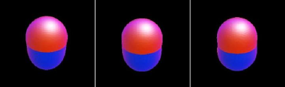
Fig. 4: Different values of line tension result different vesicle shapes.

In Figure 4, the pictures shown there correspond to equilibrium shapes with three different values of the line tension $10.0,30.0,100.0$. The bending rigidities of the blue colored component is $3.5$ while that of the red is $0.5$. By increasing the line tension, the individual components in the two-component vesicle become more hemisphere like which are the results of the increasing effect of line tension under the same volume and surface area constraints.

Figure 5 gives an even more convincing example to the rupture and vesicle fission observed in this process. As shown in Figure 5, we start from the top left shape. While preserving $v_{d}$, $a_{0}$ and $a_{d}$ to be $-213.98$, $29.46$ and $-13.31$ respectively, we increase significantly the line tension from $10.0$ to $100.0$. The vesicle gradually breaks its vertical symmetry and a small blue vesicle is separated and eventually absorbed into the top portion through a process like Oswald ripening. Finally, the vesicle (bottom-right picture of Figure 5) only contains two parts, much like the shape observed in the experiments [2].

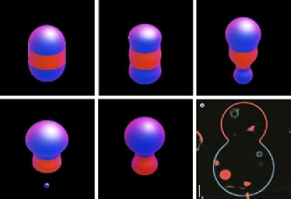
Fig. 5: Effect of line tension: rupture and fission of vesicles components (the right bottom picture is reproduced from [2]).

Comparison with other experimental results.

We now focus on the simulations that mimic other two-component vesicle shapes observed in the experiments of [2], similar to the results depicted in Figures 3 and 5.

As shown in the two rows of Figure 6, we carry out two simulations starting from a shape given on the left. In both simulations, the red component has bending rigidity $3.0$, and the blue component has bending rigidity $1.0$. The line tension between two components is $30.0$. The parameter $v_{d}$ for volume constant is $-218.00$, and the surface area parameter $a_{0}$ is $29.46$. The parameter $a_{d}$ giving the difference of surface areas of the two components takes on the values $18.76$ and $-18.76$ respectively. The final shapes of the two simulations are shown in the center pictures in both rows. One can compare them with the right most experimental picture provided in [2].

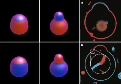
Fig. 6: Similar membrane shapes with different areas for the two components (the pictures on the right column are reproduced from [2]).

Energy	$E_{r}$	$E_{b}$	$E_{r}+E_{b}$	$E_{l}$	$E_{r}+E_{b}+E_{l}$
Top	58.36	12.15	70.51	138.17	208.68
Bottom	34.83	20.06	54.89	138.01	192.90

Table 3: Energy comparison for the shapes given in Figure 6.

The energy values of the two experiments illustrated in Figure 6 are given in Table 3 with energy contributions listed for individual components and the line tension from the phase boundary. We get almost the same line tension energy contribution, but, as caused by the difference in the bending rigidities, the elastic bending energy contributions differ by a factor of 3, which is reflective of the ratio of the bending rigidities.

We now turn to simulate a couple of other interesting shapes experimentally observed in [2] as illustrated in the last pictures of Figure 7 and Figure 10 respectively. In Figure 7, we first start from a spherical surface which is divided into two components where one component occupies similar spherical caps in twelve well-spaced locations on the membrane surface. The bending rigidity is $3.5$ for the red component and $0.5$ for the blue component, and the line tension is $10.0$. With a larger surface area of the blue component and a smaller volume than those values for the exact sphere, the blue component (with smaller bending rigidity) starts to bulge. The parameters are taken respectively as $v_{d}=-174.17$, $a_{0}=54.63$ and $a_{d}=11.01$. If we further increase the volume and enlarge the relative area of the blue component by increasing $v_{d}$ to $-167.00$, while keeping $a_{0}$ at $54.63$ and changing $a_{d}$ to $5.00$, the resulting computed shape (the third picture in Figure 7) is very similar to the experiment findings [2] (the last picture in Figure 7).

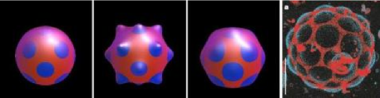
Fig. 7: A sphere with disk like bumps: comparing with biological experiments.

The shape corresponding to the third picture of Figure 7 stays as a near equilibrium (meta-stable) state for a range of parameter values. But if we further increase the area of the blue component, for example, by setting $a_{d}=2.5$, further coarsening of the blue components will take place. The merger of disconnected components continues, much like the Oswald ripening effect, and eventually transforms into shapes similar to that presented earlier in Figures 2 and 4. The transformation is illustrated in Figure 8.

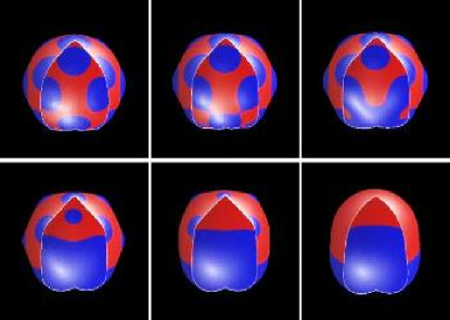
Fig. 8: The merging of blue component (cut view).

Next, we take an initial membrane profile similar to that in the second picture of Figure 7. By setting $v_{d}=-203.00$, $a_{0}=54.63$ and $a_{d}=5.00$ so that both the total volume and the area of the red components are decreased, we can then observe the growth of bumps of the red component, leading to a shape shown in the right pictures of Figure 9. Take other initial profiles, other equilibrium shapes as shown in the left and center pictures in Figure 9 have also been observed in our simulations.

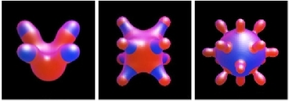
Fig. 9: Various shapes of two component membranes.

From Figure 9, it can be seen that the two-component vesicles may display very rich patterns, even in the absence of spontaneous curvature effect. One naturally may wonder if some of them are experimentally observable. The next set of experiments draws inspiration from the center and right figures of Figure 9 and leads to interesting comparisons with similar experimental observations in [2]. We start with the same phase field $\phi$ as the profile in the right picture of Figure 9, but use a modified $\eta$ such that the neck of the bumps are formed by the blue component as the case of the center picture of Figure 9. This leads to an initial shape as shown in the left picture of Figure 10. Setting the parameters as $v_{d}=-203.00$, $a_{0}=54.63$, and $a_{d}=22.68$, we finally get a shape (center picture of Figure 10) very close to the experimentally observed shape given in [2] (right picture of Figure 10).

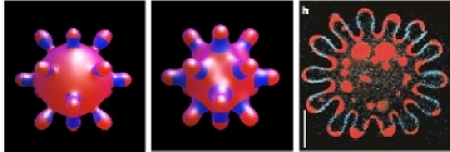
Fig. 10: Two-component shape with 14 bumps (the last picture is from [2]).

Shapes depicted in 10 are fairly robust. In fact, with a slight modification of the final shape and a rotation with a given angle, then we found that using the gradient flow, the equilibrium solution is again in the shape (except for a rotation). Results of such calculations on both $64^{3}$ and $96^{3}$ grids are given for comparison.

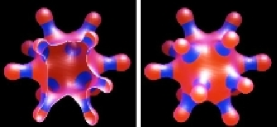
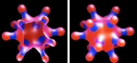
Fig. 11: Rotated two-component shapes with 14 bumps computed by different meshes.

4 Open liposomal membranes

In this section, we apply similar ideas to model open lipid membranes. The transformations from vesicles to open membranes and the reverse process from open membranes to vesicles were first observed in [30]. Here, we only consider the one-component open membranes with specified surface areas. The total energy of an open membrane $\Gamma$ with edge $\gamma_{0}$ may be conveniently defined as the sum of the elastic bending energy and the line tension energy [8, 33, 34, 35, 37]:

$$\int_{\Gamma}\left(a_{1}+a_{2}(H-c_{0})^{2}+a_{3}G\right)\,ds+\int_{\gamma_{0}}\delta\,dl\;.$$

For simplicity, we set the surface tension $a_{1}$ and the line tension $\delta$, as two constants, we also do not consider the contribution of the geodesic curvature term in the line energy on the boundary. The effects of surface tension, the Gaussian and spontaneous curvatures are also ignored. Our problem is then to minimize the following total energy

$$E_{o}=\int_{\Gamma}kH^{2}\,ds+\int_{\gamma_{0}}\delta\,dl$$

with prescribed surface area $|\Gamma|$.

Most of the available numerical simulations for open membranes have largely been confined to axis-symmetric cases based on the variational calculation of the above energy. We hereby develop a new phase field model for open membranes, and present some numerical simulations for the full three dimensional case to demonstrate the effectiveness of the model.

Phase field model for open membranes.

We can treat open membranes as two component membranes with one component having zero bending rigidity. Again, we let $\gamma_{0}$ be the intersection of two orthogonal surfaces $\Gamma$ and $\Gamma_{0}$ which are implicitly defined as the level-set of the functions $\phi$ and $\eta$ respectively.

Now we denote $c(\eta)=\frac{1}{2}(1+\tanh(\frac{\eta}{\xi}))$, and let the line tension energy be still formulated by $L(\phi,\eta)$ in (4), with the elastic bending energy of the membrane

$$E(\phi,\eta)=\int_{\Omega}\frac{kc(\eta)}{2\epsilon}\big{(}\epsilon\Delta\phi+\frac{1}{\epsilon}\phi(1-\phi^{2})\big{)}^{2}\,dx,$$

Then, our phase field model for open membranes is to minimize $E(\phi,\eta)+L(\phi,\eta)$ with the surface area constraint

$$D(\phi,\eta)=\int_{\Omega}c(\eta)[\frac{\epsilon}{2}|\nabla\phi|^{2}+\frac{1}{4\epsilon}(\phi^{2}-1)^{2}]\,dx=a_{d}\;.$$ (17)

Similar to the two-component vesicle case studied earlier, to maintain the good profiles for both phase field functions $\phi$ and $\eta$ and the orthogonality of $\Gamma$ and $\Gamma_{\perp}$, we can again take the penalty formulation

$${\cal E}_{M}(\phi,\eta) = W(\phi,\eta)+L(\phi,\eta)+\frac{1}{2}M_{3}(D(\phi,\eta)-a_{d})^{2}$$ (18)

$$+\frac{1}{2}M_{4}(N(\phi,\eta))^{2}+\frac{1}{2}M_{5}(P(\eta))^{2}+\frac{1}{2}M_{6}(P(\phi))^{2}\;.$$

Then, we can again use a gradient flow like (16) to compute the equilibrium shapes by a similar numerical scheme as that given in section 3.

Numerical simulations of open membranes

We now present some numerical simulations of open membranes and compare them with biological experimental findings. Most of the model and simulation parameters are chosen to be in the same range as that for the two component vesicle simulations in the earlier section.

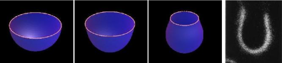
Fig. 12: Open membranes with different line tensions (the right most picture is reproduced from [30]).

Figure 12 gives the simulation results of a simple open membrane. Starting from a half sphere (the left picture), with bending rigidity $k=1.0$ and line tension $\delta=1.0$, we get an equilibrium shape shown in the second picture. If a larger line tension $\delta=1.28$ is used, an equilibrium shape is reached as that in the third picture. One can compare it with the right picture obtained in the biological experiments described in [30]. We note that the elastic bending energy are $10.12$ and $15.96$ and the line tension energy are $10.94$ and $7.95$ respectively for the solutions in the second and third pictures.

The time evolution snapshots are given in Figure 13 where the line tension is taken as $\delta=25.0$. The simulation results show that, when the line tension becomes large enough, the open membrane becomes self-enclosed.

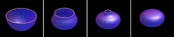
Fig. 13: Open membrane closes due to large line tension.

Finally, in Figure 14, we simulate a shape (the right picture) with three holes as observed in an experiment of [30]. Starting from the left most picture corresponding to an ellipsoid with three holes, setting the bending rigidity $k=1.0$ and line tension $\delta=1.0$, and following the gradient flow of the energy, the initial shape starts to deform first into an intermediate shape given in the second picture. The computed equilibrium shape is shown in the third picture which again shows striking similar to the experimental finding.

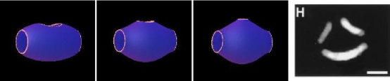
Fig. 14: Open membranes with three holes (the right most picture is reproduced from [30]).

5 Conclusion

In this paper, we formulated a phase field model for the multi-component vesicles membranes, and as a special case, the open membranes with free edges. The models incorporate the effect of the elastic bending energy together with the line tension between each two components. Full three dimensional numerical simulations presented here demonstrate that the experimental observations given in [2] can be effectively simulated by the phase field bending elasticity and line tension model. Furthermore, the simulation results illustrate that many experimentally observed exotic patterns such as bud formation and vesicle fission can appear in two-component vesicles due to the inhomogeneous bending stiffness and the competition of the bending energy and the interfacial line tension even without incorporating the spontaneous curvature or the asymmetry of the bilayer.

In conclusion, we point out the this generalization of our diffusive interface model to two component vesicle membranes fits nicely into the previously established unified framework for the derivation of dynamic and static equations and the development of numerical algorithms and codes. Many issues remain to be examined in future works. First, there maybe other more effective ways in formulating the line tension energy, including the use of geodesic curvature along the phase boundary, which may be important to model the difference of the stretching rigidity in two components [3]. Second, more rigorous analysis of our models are needed in the future. Third, in our numerical simulations, we have not examined the effect of the spontaneous curvature as we have done for the one component case [15]. It is expected that more complex shapes would be be discovered in this case. Moreover, the interaction of multi-component vesicles with the fluid and electric fields are also exciting topics to be investigated further in the future.

Appendix: Justification of the energy and constraints.

We now provide some brief calculations to rationalize the definitions of the energy functional and the constraints in the phase field setting. Same as the discussion in [17], we can first illustrate that in a very broad ansatz, for small $\epsilon$ and $\xi$, minimizing $W(\phi,\eta)$ leads to a phase field function $\phi(x)$ which is approaching to $\tanh(d(x,\Gamma)/(\sqrt{2}\epsilon))$ as $\epsilon\rightarrow 0$. In fact for small $\epsilon$, due to the uniform bound of the functional $B$, the region away from the level set $\phi=0$ are all close to $\phi=+1$ or $-1$. In such cases, one can always define the following transformation near the interface:

$$\phi(x)=q^{\epsilon}(\frac{d(x)}{\epsilon}),$$ (19)

where $d(x)$ is the distance of the point $x\in\Omega$ to the surface $\Gamma$. Substituting this into (3), we have that:

$$E(\phi)=\int_{\Omega}\frac{k(\eta)}{2\epsilon}\left|{q^{\epsilon}}^{\prime}(\frac{d(x)}{\epsilon})\Delta d(x)+\frac{1}{\epsilon}({q^{\epsilon}}^{\prime\prime}-({q^{\epsilon}}^{2}-1)q^{\epsilon})\right|^{2}\,dx.$$ (20)

If we keep $k(\eta)$ positive, as $\epsilon\rightarrow 0$, to minimize the energy, the leading term in the above has to vanish, that is,

$$\left|{q^{\epsilon}}^{\prime\prime}-({q^{\epsilon}}^{2}-1)q^{\epsilon}\right|^{2}\rightarrow 0$$ (21)

which means that the transition region profile $q^{\epsilon}(\cdot)$ is approaching to the function $\tanh({\frac{\cdot}{\sqrt{2}}})$. In the meantime, we see that $\phi$ is approaching to the Heaviside function with $1$ inside of the interface and $-1$ outside. $\Gamma$ still coincides with the zero level set of $\phi$. Moreover (19) indicates that the parameter $\epsilon$ is effectively the thickness of the transition region between $\{\phi=1\}$ and $\{\phi=-1\}$. One can refer [14] for more rigorous proof of this.

Now, we denote $s(\phi)=\frac{\epsilon}{2}|\nabla\phi|^{2}+\frac{1}{4\epsilon}(\phi^{2}-1)^{2}$. When the line tension $L(\phi,\eta)$ reach its minimum, we have

$$\frac{\delta L}{\delta\eta}=f(\eta,s)=-\epsilon\nabla\cdot(s\nabla\eta)+\frac{1}{\epsilon}s(\eta^{2}-1)\eta=0.$$

For $\phi=\tanh(d/(\sqrt{2}\epsilon))$, $s=\frac{1}{2\epsilon}(\phi^{2}-1)^{2}$ and therefore $\nabla s\cdot\nabla\eta=0$ as $\nabla\phi\cdot\nabla\eta=0$. Then $f(\eta,s)=0$ means

$$-\epsilon\Delta\eta+\frac{1}{\epsilon}(\eta^{2}-1)\eta=0\;.$$

If we write $\eta$ again by $q^{\epsilon}(d(x,\Gamma_{\bot})/\epsilon)$, from the above equation we have

$$-{q^{\epsilon}}^{\prime}(\frac{d}{\epsilon})\Delta d(x)+\frac{1}{\epsilon}\big{(}({q^{\epsilon}}^{2}-1)q^{\epsilon}-{q^{\epsilon}}^{\prime\prime}\big{)}=0.$$

As $\epsilon\rightarrow 0$, we have $({q^{\epsilon}}^{2}-1)q^{\epsilon}-{q^{\epsilon}}^{\prime\prime}=0$. To minimize $L$, we can expect that far away from the $\Gamma_{\bot}$, $q^{\epsilon}$ is $+1$ or $-1$, therefore we also have $q^{\epsilon}(x)=\tanh(\frac{x}{\sqrt{2}\epsilon})$. On the other hand, we can use the same argument for $\phi$ if we know $\eta$ is a tanh function, which would further strengthen the ansatz that $\phi$ and $\eta$ are both tanh functions to lead order of $\epsilon$. In fact, following more careful analysis as those in [14], we expect that the differences between $\phi$ and $\eta$ and the respective tanh profiles are second order in $\epsilon$ which would allow us to rigorous derive the asymptotic limits (8-10).

References

- [1] D. Anderson, G. McFadden and A. Wheeler, Diffusive-interface methods in fluid mechanisms, Ann. Rev. Fluid Mech. 30, pp. 139-165, 1998.
- [2] T. Baumgart, S. Hess and W. Webb, Imaging coexisting fluid domains in biomembrane models coupling curvature and line tension, Nature, Vol 425, pp. 821–824, 2003.
- [3] T. Baumgart, S. Hess, W. Webb and T. Jenkin, Membrane Elasticity in Giant Vesicles with Fluid Phase Coexistence, Biophysical Journal, 89, pp.1067-1080, 2005.
- [4] D. Benvegnu and M. McConnell, Line tension between liquid domains in lipid monolayers, Journal of Physical Chemistry, 96, pp. 6820-6824, 1992.
- [5] T. Biben, K. Kassner and C. Misbah, Phase-field approach to 3D vesicle dynamics, Phys. Rev. E., 72, pp.041921, 2005.
- [6] W. Boettinger, J. Warren, C. Beckermann, and A. Karma, Phase-field simulation of solidification, Annual Review of Materials Research, 32, pp.163-194, 2002
- [7] P. Burchard, L.-T. Cheng, B. Merriman and S. Osher, Motion of Curves in Three Spatial Dimensions Using a Level Set Approach, Journal of Computational Physics, 170, pp.720-741, 2001.
- [8] R. Capovilla, J. Guven and J. Santiago, Lipid membranes with an edge, Phys. Rev. E, 66, pp.021607, 2002.
- [9] G. Caginalp and X. F. Chen, Phase field equations in the singular limit of sharp interface problems, in On the evolution of phase boundaries (Minneapolis, MN, 1990–91), Springer, New York, 1992, pp. 1–27.
- [10] L.-Q. Chen, Phase-field models for microstructure evolution, Annual Review of Materials Research, 32, pp. 113-140, 2002.
- [11] P. G. Ciarlet, Introduction to linear shell theory, V. 1 of Series in Applied Mathematics (Paris), Gauthier-Villars, Éditions Scientifiques et Médicales Elsevier, Paris, 1998.
- [12] , Mathematical elasticity. V.III, V. 29 of Studies in Mathematics and its Applications, North-Holland Publishing Co., Amsterdam, 2000. Theory of shells.
- [13] H. Döbereiner, J. Käs, D. Noppl, I. Sprenger and E. Sackmann, Budding and fission of vesicles, Biophysical Journal, 65, pp. 1396 C1403, 1993.
- [14] Q. Du, C. Liu, R. Ryham and X. Wang, A phase field formulation of the Willmore problem, Nonlinearity, 18, pp. 1249-1267, 2005.
- [15] Q. Du, C. Liu, R. Ryham and X. Wang, Modeling the Spontaneous Curvature Effects in Static Cell Membrane Deformations by a Phase Field Formulation, Communications in Pure and Applied Analysis, 4, pp. 537-548, 2005.
- [16] Q. Du, C. Liu, R. Ryham and X. Wang, Modeling Vesicle Deformations in Flow Fields via Energetic Variational Approaches, preprint, 2006.
- [17] Q. Du, C. Liu, and X. Wang, A phase field approach in the numerical study of the elastic bending energy for vesicle membranes, Journal of Computational Physics, 198, pp. 450-468, 2004.
- [18] Q. Du, C. Liu, and X. Wang, Retrieving Topological Information For Phase Field Models, SIAM Journal on Applied Mathematics 65, pp. 1913-1932, 2005.
- [19] Q. Du, C. Liu, and X. Wang, Simulating the Deformation of Vesicle Membranes under Elastic Bending Energy in Three Dimensions, Journal of Computational Physics, 212, pp. 757-777, 2006.
- [20] W. Gozdz and G. Gompper, Shapes and shape transformations of two-component membranes of complex topology, Phys. Rev. E 59, 4305-4316 (1999).
- [21] Y. Jiang, T. Lookman, and A. Saxena, Phase separation and shape deformation of two-phase membranes, Phys. Rev. E. 6 (2000), R57-R60.
- [22] F. Juelicher and R. Lipowsky, Shape transformations of vesicles with intramembrane domains, Phys. Rev. E. 53, 2670-2683, 1996.
- [23] P. Kumar, G. Gompper and R. Lipowsky, Budding Dynamics of Multicomponent Membranes, Physical Review Letters, 86, pp.3911-3914 , 2001
- [24] R. Lipowsky, Budding of membranes induced by intramembrane domains, Journal de Physique II, France 2, pp. 1825-1840, 1992.
- [25] R. Lipowsky, The morphology of lipid membranes, Current Opinion in Structural Biology, 5, pp. 531–540, 1995.
- [26] R. Lipowsky, Domains and Rafts in Membranes Hidden Dimensions of Self-organization, Journal of Biological Physics, 28, pp.195-210, 2002.
- [27] J. McWhirter, G. Ayton and G. Voth, Coupling Field Theory with Mesoscopic Dynamical Simulations of Multicomponent Lipid Bilayers, Biophysical Journal 87, pp. 3242-3263, 2004.
- [28] Z. Ou-Yang, J. Liu, and Y. Xie, Geometric Methods in the Elastic Theory of Membranes in Liquid Crystal Phases, World Scientific, Singapore, 1999.
- [29] S. Osher and R. Fedkiw, The Level Set Method and Dynamic Implicit Surfaces, Springer-Verlag, 2002.
- [30] A. Saitoh, K. Takiguchi, Y. Tanaka and H. Hotani, Opening-up of liposomal membranes by talin, Proceedings of the National Academy of Sciences, Biophysics, 956, pp. 1026-1031, 1998.
- [31] U. Seifert, Curvature-induced lateral phase separation in two-component vesicles, Physical Review Letters, 70, pp. 1335-1338, 1993.
- [32] J. A. Sethian. Level Set Methods and Fast Marching Methods: evolving interfaces in computational geometry, fluid mechanics, computer vision, and materials science. Cambridge University Press, New York, 2nd edition, 1999.
- [33] Z. Tu and Z. Ou-Yang, Lipid membranes with free edges, Physical Review E, 68, 061915 (1-7), 2003.
- [34] Z. Tu and Z. Ou-Yang, A geometric theory on the elasticity of bio-membranes, Journal of Physics A: Mathematical and General, 37, pp. 11407-11429, 2004.
- [35] T. Umeda, Y. Suezaki, K. Takiguchi, and H. Hotani, Theoretical analysis of opening-up vesicles with single and two holes, Phys. Rev. E, 71, pp.011913 (1-8), 2005.
- [36] X. Wang, Phase Field Models and Simulations of Vesicle Bio-membranes, Ph.D thesis, Department of Mathematics, Penn State University, 2005.
- [37] Y. Yin, J. Yin and D. Ni, General Mathematical Frame for Open or Closed Biomembranes I: Equilibrium Theory and Geometrically Constraint Equation, Journal of Mathematical Biology, 51, pp. 403-413.