Boolean Game on Scale-free Networks

Abstract

Inspired by the local minority game, we propose a network Boolean game and investigate its dynamical properties on scale-free networks. The system can self-organize to a stable state with better performance than random choice game, although only the local information is available to the agent. By introducing the heterogeneity of local interactions, we find the system has the best performance when each agent’s interaction frequency is linear correlated with its information capacity. Generally, the agents with more information gain more than those with less information, while in the optimal case, each agent almost has the same average profit. In addition, we investigate the role of irrational factor and find an interesting symmetrical behavior.

1 Introduction

In recent years, the phenomena of collective behavior related to populations of interacting individuals attract increasing attentions in the studies on scientific world, especially in the economical and biological systems [1, 2, 3]. To describe and explain the self-organized phenomenon, many models are established. Inspired by Arthur’s Farol Bar Problem [4], Challet and Zhang proposed the so-called minority game (MG) [5, 6], which is a simple but rich model showing how selfish agents fight for common resources in the absence of direct communication.

In the standard minority game, a group of $N$ (odd) agents has to choose between two opposing actions, which are labelled by $+1$ and $-1$ , respectively. In the real systems of stock market, these options mean to buy stock or to sell. Each agent is assigned a set of $s$ strategies and informed the updated global outcomes for the past $M$ time steps. At each time step, they use the most working strategies to make decisions, and those who end up in the minority side (the side chosen by fewer agents) win and get a point. Though simple, MG displays the self-organized global-cooperative behaviors which are ubiquitously observed in many social and economic systems [7, 8, 9, 10, 11, 12, 13, 14, 15, 16, 17]. Furthermore, it can explain a large amount of empirical data and might contribute to the understanding of many-body ecosystems [18, 19, 20].

In the real world, an individual ia able to get information from his/her acquaintances, and try to perform optimally in his/her immediate surroundings. In order to add this spatial effect to the basic MG, recently, some authors introduced the so-called local minority game (LMG), where agent could make a wiser decision relying on the local information [21, 22, 23, 24, 25, 26, 27]. It is shown that the system could benefit from the spatial arrangement, and achieves self-organization which is similar to the basic MG.

Denote each agent by a node, and generate a link between each pair of agents having direct interaction, then the mutual influence can vividly be described by means of the information networks. Accordingly, node degree $k$ is proportional to the quantity of information available to the corresponding agent. Most LMG models are based on either the regular networks, or the random ones. Nevertheless, both of them have a characterized degree, the mean degree $\langle k\rangle$, which means each agent is almost in the same possession of information. However, previous studies reveal that the real-life information networks are highly heterogeneous with approximately power-law distributions [28, 29, 30]. Thus the above assumption is quite improper for the reality. In common sense, those who process huge sources of information always play active and important roles. Therefore, in this paper, we will study the case on the base of scale-free networks.

Another interesting issue is the herd behaviors that have been extensively studied in Behavioral Finance and is usually considered as a crucial origin of complexity that enhances the fluctuation and reduces the system profit [32, 33, 34, 35, 36, 37]. Here we argue that, to measure the potential occurrence of herd behavior, it is more proper to look at how much an agent’s actions are determined by others (i.e. the local interaction strength of him) rather than how much he wants to be the majority. It is because that in many real-life situations, no matter how much the agents want to be the minority, the herd behavior still occurs. To reveal the underlying mechanism of the herd behavior, three questions are concerned in this paper:

a) Whether agents have different responses under the same interaction strength?

b) What are the varying trends of individual profit as the increase of interaction strength?

c) What are the effects of heterogenous distribution of individual herd strength on system profit?

Furthermore, a fundamental problem in complexity science is how large systems with only local information available to the agents may become complex through a self-organized dynamical process [31, 38]. In this paper, we will also discuss this issue based on the present model by detecting the profit-degree correlations.

2 Model

In the present model, each agent chooses between two opposing actions at each time step, simplified as +1 and -1. And the agents in the minority are rewarded, thus the system profit equals to the number of winners [6, 9]. At each time step, each agent $x$ will, at probability $p_{x}$, make a call to one randomly selected neighbor to ask about this neighbor’s last action, and then decide to choose the opposing one; or at probability $1-p_{x}$, agent $x$ simply inherits his previous action. Accordingly, in the former case, agent $x$ will choose +1 at a probability $\frac{s_{-1}^{x}}{s_{-1}^{x}+s_{+1}^{x}}$, or choose -1 at a probability $\frac{s_{+1}^{x}}{s_{-1}^{x}+s_{+1}^{x}}$, where $s_{+1}^{x}$ and $s_{-1}^{x}$ denote the number of $x$’s neighbors choosing +1 and -1 in the last time step, respectively. It is worthwhile to emphasize that the agents do not know who are the winners in the previous steps since the global information is not available. This is one of the main distinctions from the previously studied LMG models.

Take the irrational factor into account [35], each agent may, at a mutation probability $m$, choose an opposite action. The mutation probability adds several impulsive and unstable ingredients to our model. Just as the saying goes, ‘nothing is fixed in the stone’, actually, people can not consider every potential possibility that would come out when making a decision. So, it is the case that we are making the mind at this moment and changing our mind at the next. To this extent, the introduction of the mutation parameter enriches the model.

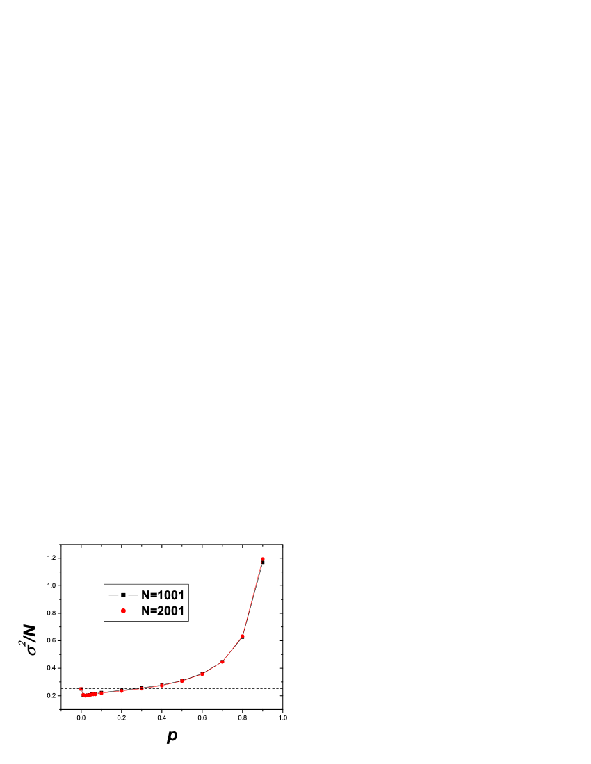
Figure 1: (Color online) The normalized variance as a function of the average interaction strength $p$ on the BA network of size 1001 and size 2001. The dashed line represents the system profit of random game. The system performs better than the random game when $p\in(0,0.28)$. Besides, the two curves are almost the same, indicating the present $\frac{\sigma^{2}}{N}-p$ relationship does not depend on the system size $N$.

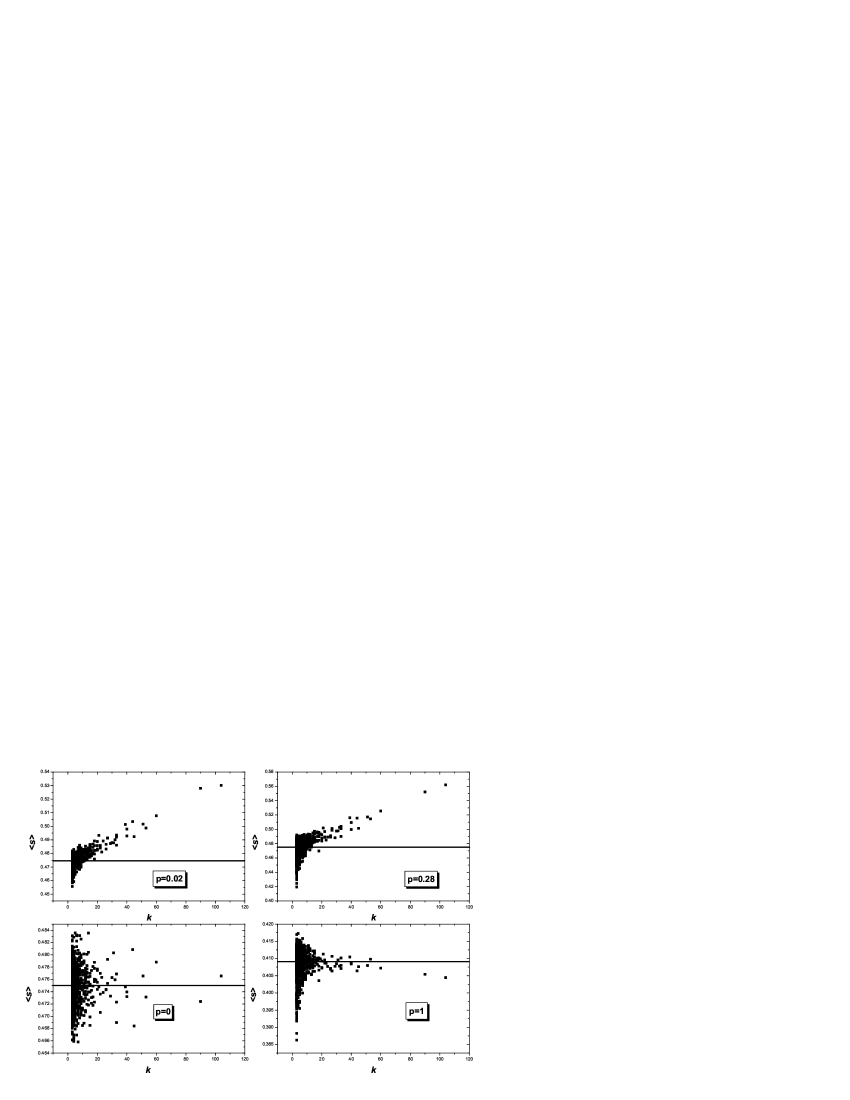
Figure 2: The agent’s winning rate versus degree. Each data point denotes one agent and the solid line represents the average winning rate of all the agents. The cases $p=0$ and $p=1.0$ correspond to the completely independent and dependent cases, respectively; $p=0.02$ is the point where the system performs best, and $p=0.28$ is another point where the system profit is equal to the random game.

Considering the potential relationship between individual’s information capacity and herd strength, we assume $p_{x}\sim k_{x}^{\beta}$, where $k_{x}$ is $x$’s degree, and $\beta$ is a free parameter. Denote $p=\frac{1}{N}\sum_{x}p_{x}$ the average herd strength, then one has

$$p_{x}=Np\frac{k_{x}^{\beta}}{\sum_{y}k_{y}^{\beta}},$$ (1)

where the subscript $y$ goes over all the nodes.

There are three cases for interaction strength distributions.

a) $\beta=0$, each agent of the network shares the same interaction strength $p$.

b) $\beta>0$, heterogeneity occurs: The greater the degree, the stronger the interaction strength, that is, hub nodes depend on the local information while small nodes exhibit relatively independent decision making.

c) $\beta<0$, the heterogeneity occurs in the opposite situation: The smaller the degree, the stronger the interaction strength, that is, hub nodes exhibit independence while small nodes depend on the local information.

The special case with $m=0.01$ and $\beta=0$ has been previously studied to show the effect of degree heterogeneity on the dynamical behaviors [39].

3 Simulation and Analysis

3.1 Self-organized phenomenon

In this paper, all the simulation results are averaged over 100 independent realizations, and for each realization, the time length is $T=10000$ unless some special statement is addressed. The Barabási-Albert (BA) networks with minimal degree $m=3$ are used [40, 41]. Initially, each node randomly choose $+1$ or $-1$. In this subsection, we concentrate on the case $\beta=0$ and $m=0.01$.

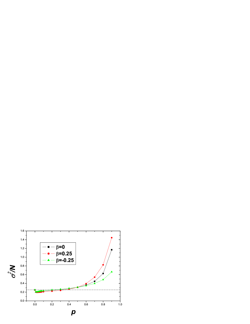
Figure 3: (Color online) The normalized variance as a function of the average interaction strength $p$. The dashed line represents the system profit of random game. The system performs better than random game when $p\in(0,0.2)$, $p\in(0,0.28)$ and $p\in(0,0.34)$ for $\beta=-0.25$, $\beta=0$ and $\beta=0.25$, respectively.

The performance of the system can be measured by the variance $\sigma^{2}=(1/T)\Sigma_{t=1}^{T}(A_{t}-N/2)^{2}$, where $A_{t}$ is the number of agents who choose +1 at time step t, and $N$ denotes the network size [6, 9, 17]. Clearly, smaller $\sigma^{2}$ corresponds to more system profit and for the completely random choice game (random game for short), $\sigma^{2}=0.25N$. Fig. 1 shows the normalized variance $\frac{\sigma^{2}}{N}$ as a function of the average interaction strength $p$ (Since $\beta=0$, all the nodes have the same interaction strength $p$). Unexpectedly, although the global information is unavailable, the system is able to perform better than random game in the interval $p\in(0,0.28)$. This is a strong evidence for the existence of self-organized process. In addition, we attain that the network size effect is very slight for sufficient $N$ ($N\sim 10^{3}$), thus hereinafter, only the case $N=1001$ is investigated.

In Fig. 2, we report the agent’s winning rate versus degree, where the winning rate is denoted by the average score $\langle s\rangle$ during one time step. Obviously, unless the two extreme points $p=0$ and $p=1$, there is a positive correlation between the agent’s profit and degree, which means the agents of larger degree will perform better than those of less degree. If the agents choosing $+1$ and $-1$ are equally mixed up in the network, there is no correlation between profit and degree [39]. Therefore, this positive correlation provides another evidence of the existence of a self-organized process.

3.2 Effect of interaction strength heterogeneity on system profit

In this subsection, we investigate how $\beta$ affects the system profit with mutation probability $m=0.01$ fixed.

In Fig. 3, it is observed that in all the three cases $\beta=-0.25,\beta=0,$ and $\beta=0.25$, the system performs more efficiently than the random choice game when $p$ is at a certain interval. More interesting, when the interaction strength $p$ is small ($p<0.5$), the system with positive $\beta$ ($\beta=0.25$) performs best, while for large $p$ ($p>0.5$), the system with negative $\beta$ ($\beta=-0.25$) performs best. However, this phenomenon does not hold if $|\beta|$ is too large ($\beta\cong 1$).

We have checked that for all the cases with $\beta\in(-1,1)$, all the systems achieve their own optimal state at the interval $p\in[0.02,0.1]$. When given $p$, it is natural to question whether there exists an optimal $\beta$, in which the system performs best. We report the normalized variance as a function of $\beta$ for different $p$ in figure 4. Remarkably, all the optimal states are achieved around $\beta=1$. Besides, it is worthwhile to attach significant importance to the case when $\beta=1$ and $p=0.08$, when we have the most profitable system.

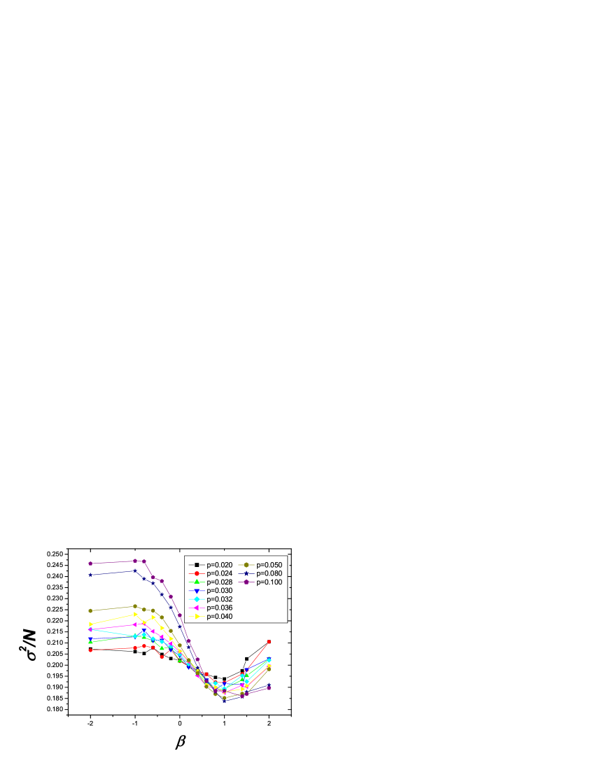
Figure 4: (Color online) the normalized variance as a function of the interaction power $\beta$ for several selected $p$ indicated in the inset. Evidently, the system tends to perform optimally when the interaction power $\beta$ is around 1.

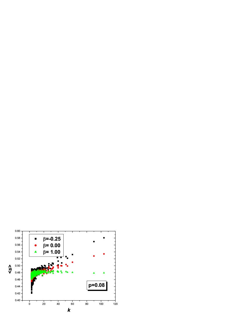
Figure 5: (Color online) The agent’s winning rate versus degree, where each data point corresponds to one agent. The black squares, red circles and green triangles denote the case $\beta=-0.25$, $\beta=0$ and $\beta=1$, respectively.

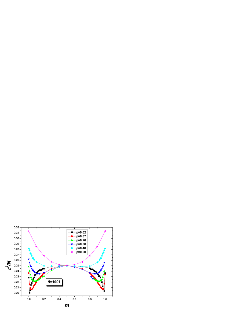
Figure 6: (Color online) The normalized variance as a function of the mutation probability $m$ for several selected $p$. The parameter $\beta=0$ is fixed. Obviously, the curves exhibit symmetry with a dividing point $m=0.5$. When $m=0.5$, every system has the same profit as the random game though different $p$. The shapes of these curves vary as $p$ increases: For small $p$, the curves have the peculiar “two-winged” shape, while for large $p$, the curves become U-shaped. The cases for $p>0.5$ have very large $\sigma^{2}/N$ when $m$ is close to 0 or 1, thus not shown here.

The interaction strength heterogeneity can have some positive effects on system as a whole, including better use of the information and more profit. We wonder which group of people profit after all? Specifically, figure 5 shows the agent’s winning rate versus degree for $\beta=-0.25$, 0 and 1, where $p=0.08$ is fixed. Unexpectedly, in the most optimal system (i.e. $\beta=1$ and $p=0.08$), the profit-degree correlation vanishes. So one may draw an interesting conclusion that the great disparity between poor and rich population is not the necessary condition for an efficient social. However, we can not give an analytical solution about this phenomenon, and the corresponding conclusion may be only valid for this special model.

3.3 Role of irrational factor

Figure 6 reports the normalized variance as a function of the mutation probability $m$. Interestingly, the curves display symmetry with a dividing point $m=0.5$ at which each system has the same profit as the random game. For arbitrary agent, denote $s_{a}$ the number of this agent’s neighbors choosing $a$ in the present time step, and $p_{(a,b)}$ the probability he/she will choose $b$ in the next time step under the condition that he/she chooses $a$ in the present time step. Clearly, one has

$$p_{(+1,+1)}=\frac{(1-m)p\cdot s_{-1}}{s_{-1}+s_{+1}}+\frac{m\cdot p\cdot s_{+1}}{s_{+1}+s_{-1}}+(1-m)(1-p)\\$$ (2)

$$p_{(+1,-1)}=\frac{(1-m)p\cdot s_{+1}}{s_{-1}+s_{+1}}+\frac{m\cdot p\cdot s_{-1}}{s_{+1}+s_{-1}}+m(1-p)$$ (3)

$$p_{(-1,+1)}=\frac{(1-m)p\cdot s_{-1}}{s_{-1}+s_{+1}}+\frac{m\cdot p\cdot s_{+1}}{s_{+1}+s_{-1}}+m(1-p)$$ (4)

$$p_{(-1,-1)}=\frac{(1-m)p\cdot s_{+1}}{s_{-1}+s_{+1}}+\frac{m\cdot p\cdot s_{-1}}{s_{+1}+s_{-1}}+(1-m)(1-p)$$ (5)

If $m=0.5$, $p_{(+1,+1)}=p_{(+1,-1)}=p_{(-1,+1)}=p_{(-1,-1)}=0.5$ (the same as that of the random game), thus $\sigma^{2}/N=0.25$ (independent of $p$). Additionally, replace $m$ by $1-m$, one will immediately find the symmetry.

4 Conclusion

In summary, inspired by the local minority game, we propose a network Boolean game. The simulation results upon the scale-free network are shown. The system can self-organize to a stable state with a better performance than the random choice game, although only the local information is available to the agent. This is a reasonable evidence of the existence of a self-organized process. We find remarkable differences between the case with local interaction strengths identical for all agents ($\beta=0$), and that with local interaction strengths unequally distributed to the agents. The interval of $p$, within which the system can perform better than the random game, is obviously extended in the case when $\beta>0$. In addition, the system reaches the best performance when each agent’s interaction frequency is linear correlated with its information capacity. Generally, the agents with more information gain more, however, in the optimal case, each agent has almost the same average profit. Within the frame of this model, the great disparity between poor and rich population is not the necessary condition for an efficient social. The effect of irrational factor on the dynamics of this model is also investigated, and an interesting symmetrical behavior is found.

Although is rough, the model offers a simple and intuitive paradigm of many-body systems that can self-organize even when only local information is available. Since the self-organized process is considered as one of the key ingredients of the origins of complexity, hopefully, the model as well as its perspectives and conclusions might contribute to the achievement of the underlying mechanism of the complex systems. Furthermore, using the method proposed by Challet, Marsili, and Zhang [42, 43, 44], the market price can be introduced to the present model by define the price return proportional to the difference between the numbers of agents choosing $+1$ and $-1$. In this sense, one is able to check if this model can display stylized facts in accordance with the real markets.

Finally, we would like to point out that to set some kinds of action strength correlated with the degree of corresponding node in a power-law form (e.g. $p_{x}\sim k_{x}^{\beta}$) to better the system performance is not only available in this particular issue, but also a widely used approach for many dynamics upon scale-free networks, such as to fasten searching engine [45] and broadcasting process [46], to enhance network synchronizability [47], to improve traffic capacity [48], and so on. We believe this method can also be applied to the studies on many other network dynamical processes.

References

- [1] R.N. Mantegna, H.E. Stanley, Introduction to Econophysics: Correlations and Complexity in Finance, Cambridge University Press, Cambridge, 1999.
- [2] J.-P. Bouchaud, M. Potters, Theory of Financial Risks, Cambridge University Press, Cambridge, 2000.
- [3] L.Lam, Nonlinear Physics for Beginners, World Scientific Press, River Edge, N J, 2000.
- [4] W.B. Arthur, Am. Econ. Rev. (Papers and Proceedings) 84 (1994) 406.
- [5] D. Challet, Y.C.Zhang, Physica A 246 (1997) 407.
- [6] D. Challet, Y.C.Zhang, Physica A 256 (1998) 514.
- [7] N.F. Johnson, M. Hart, P.M. Hui, Physica A 269 (1998) 1.
- [8] M. Marsili, Physica A 299 (2001) 93.
- [9] R. Savit, R. Manuca, R. Riolo, Phys. Rev. Lett 82 (1999) 2203.
- [10] Y.-B. Xie, B.-H. Wang, C.-K. Hu, T. Zhou, Eur. Phys. J. B 47 (2005) 587.
- [11] M.A.R. de Cara, O. Pla, F. Guinea, Eur. Phys. J. B 10 (1999) 187.
- [12] M.A.R. de Caram O. Pla, F. Guinea, Eur. Phys. J. B 13 (2000) 413.
- [13] Y. Li, R. Riolo, R. Savit, Physica A 276 (2000) 234.
- [14] Y. Li, R. Riolo, R. Savit, Physica A 276 (2000) 265.
- [15] R. D’hulst, G.J. Rodgers, Physica A 270 (1999) 514.
- [16] R. D’hulst, G.J. Rodgers, Physica A 278 (2000) 579.
- [17] H.-J. Quan, B.-H. Wang, P.-M. Hui, Physica A 312 (2002) 619.
- [18] N.F. Johnson, S. Jarvis, R.Jonson, P. Cheung, Y.R. Kwong, P.M. Hui, Physica A 258 (1998) 230.
- [19] N.F. Johnson, P.M. Hui, D. Zheng, C.W. Tai, Physica A 269 (1999) 493.
- [20] N.F. Johnson, P.M. Hui, R. Jonson, T.S. Lo, Phys. Rev. Lett. 82 (1999) 3360.
- [21] T. Kalinowski, H.-J. Schulz, M. Briese, Physica A 277 (2000) 502.
- [22] S. Moelbert, P. De Los Rios, Physica A 303 (2002) 217.
- [23] E. Burgos, H. Ceva, R.P.J. Perazzo, Physica A 337 (2004) 635.
- [24] E. Burgos, H. Ceva, R.P.J. Perazzo, Physica A 354 (2005) 518.
- [25] H.F. Chau, F.K. Chow, Physica A 312 (2002) 277.
- [26] F.K. Chow, H.F. Chau, Physica A 319 (2003) 601.
- [27] F. Slanina, Physica A 299 (2001) 334.
- [28] R. Albert, A.-L. Barabási, Rev. Mod. Phys. 74 (2002) 47.
- [29] L. Kullmann, J. Kertész, K. Kaski, Phys. Rev. E 66 (2002) 026125.
- [30] M. Anghel, Z. Toroczkai, K.E. Bassler, G. Korniss, Phys. Rev. Lett. 92 (2004) 058701.
- [31] M. Paczuski, K.E. Bassler, Phys. Rev. Lett. 84 (2000) 3185.
- [32] V.M. Eguíluz, M.G. Zimmermann, Phys.Rev.Lett. 85 (2000) 5659.
- [33] Y.-B. Xie, B.-H. Wang, B. Hu, T. Zhou, Phys. Rev. E 71 (2005) 046135.
- [34] J. Wang, C.-X. Yang, P.-L. Zhou, Y.-D. Jin, T. Zhou, B.-H. Wang, Physica A 354 (2005) 505.
- [35] T. Zhou, P.-L. Zhou, B.-H. Wang, Z.-N. Tang, J. Liu, Int. J. Mod. Phys. B 18 (2004) 2697.
- [36] R. Cont, J.P. Bouchaud, Marcroecomonic Dynamics 4 (2000) 170.
- [37] C.-X. Yang, J. Wang, T. Zhou, J. Liu, M. Xu, P.-L. Zhou, B.-H. Wang, Chin. Sci. Bull. 50 (2005) 2140.
- [38] A. Vázquez, Phys. Rev. E 62 (2000) 4497.
- [39] T. Zhou, B. -H. Wang, P. -L. Zhou, C. -X. Yang, J. Liu, Phys. Rev. E 72 (2005) 046139.
- [40] A. -L. Barabási, R. Albert, Science 286 (1999) 509.
- [41] A. -L. Barabási, R. Albert, H. Jeong, Physica A 272 (1999) 173.
- [42] D. Challet, M. Marsili, and Y. -C. Zhang, Physica A 276 (2000) 284.
- [43] D. Challet, M. Marsili, and Y. -C. Zhang, Physica A 294 (2001) 514.
- [44] D. Challet, M. Marsili, and Y. -C. Zhang, Physica A 299 (2001) 228.
- [45] B. -J. Kim, C. N. Yoon, S. K. Han, and H. Jeong, Phys. Rev. E 65 (2002) 027103.
- [46] T. Zhou, J. -G. Liu, W. -J. Bai, G. Chen, and B. -H. Wang, arXiv: physics/0604083.
- [47] A. E. Motter, C. Zhou, and J. Kurths, Phys. Rev. E 71 (2005) 016116.
- [48] C. -Y. Yin, B. -H. Wang, W. -X. Wang, T. Zhou, and H. -J. Yang, Phys. Lett. A 351 (2006) 220.