Phase transition in ultrathin magnetic films with long range interactions

Abstract

Ultrathin magnetic films can be modeled as an anisotropic Heisenberg model with long range dipolar interactions. It is believed that the phase diagram presents three phases: A ordered ferromagnetic phase ($I$), a phase characterized by a change from out-of-plane to in-plane in the magnetization ($II$), and a high temperature paramagnetic phase ($III$). It is claimed that the border lines from phase $I$ to $III$ and $II$ to $III$ are of second order and from $I$ to $II$ is first order. In the present work we have performed a very careful Monte Carlo simulation of the model. Our results strongly support that the line separating phase $II$ and $III$ is of the $BKT$ type.

I Introduction

Since the late 80’s there has being an increasing interest in ultrathin magnetic films salamon ; majkrzak ; dutcher ; gruenberg ; saurenbach ; allenspach . This interest is mainly associated to the development of magnetic-non-magnetic multilayers for the purpose of giant magnetoresistence applications levy . In addition, experiments on epitaxial magnetic layers have shown that a huge variety of complex structures can develop in the system chapman ; daykin ; johnston ; hehn . Rich magnetic domain structures like stripes, chevrons, labyrinths and bubbles associated to the competition between dipolar long range interactions and strong anisotropies perpendicular to the plane of the film were observed experimentally. A lot of theoretical work has been done on the morphology and stability of these magnetic structures chui ; vedmedenko1 ; vedmedenko2 . Beside that, it has been observed the existence of a switching transition from perpendicular to in-plane ordering at low but finite temperature pappas ; allenspach2 ; rapini-costa-landau ; santamaria : at low temperature the film magnetization is perpendicular to the film surface, as temperature rises the magnetization flips to an in-plane configuration. Eventually the out-of-plane and the in plane magnetization become zero chui2 .

The general Hamiltonian describing a prototype for a ultrathin magnetic film assumed to lay in the $xy$ plane is santamaria

$$H=-J\sum_{<ij>}\vec{S_{i}}\cdot\vec{S_{j}}-A\sum_{i}{S_{i}^{z}}^{2}+$$ (1)

$$D\sum_{<ij>}\left[\frac{\vec{S_{i}}\cdot\vec{S_{j}}}{{r}_{ij}^{3}}-3\frac{\left(\vec{S_{i}}\cdot\vec{r}_{ij}\right)\cdot\left(\vec{S_{j}}\cdot\vec{r}_{ij}\right)}{{r}_{ij}^{5}}\right].$$

Here $J$ is an exchange interaction which is assumed to be nonzero only for nearest-neighbor interaction, $D$ is the dipolar coupling parameter, $A$ is a single-ion anisotropy and $\vec{r}_{ij}=\vec{r}_{j}-\vec{r}_{i}$ where $\vec{r}_{i}$ stands for lattice vectors. The structures developed in the system depend on the sample geometry and size. Several situations are discussed in reference vedmedenko2 and citations therein.
Although the structures developed in the system are well known the phase diagram of the model is still being studied. There are several possibilities since we can combine the parameters in many ways. We want to analyze the case $J>0$ in some interesting situations. A more detailed analysis covering the entire space of parameters is under consideration.

• Case $D=0$
  For $D=0$ we recover the two dimensional ($2d$) anisotropic Heisenberg model. The isotropic case, $A=0$, is known to present no transition mermin-wagner . For $A>0$ the model is in the Ising universality class Ising undergoing a order-disorder phase transition. If $A<0$ the model is in the $XY$ universality class. In this case it is known to have a Berezinskii-Kosterlitz-Thouless ($BKT$) phase transition which is characterized by a vortex-anti-vortex unbinding, with no true long range order berezinskii ; kosterliz-thouless ; teitel ; kogut .

• Case $D\neq 0$
  In this case, there is a competition between the dipolar and the anisotropic terms. If $D$ is small compared to $A$ we can expect the system to have an Ising behavior. If $D$ is not too small we can expect a transition of the spins from out-of-plane to in-plane configuration santamaria . For large enough $D$ out-of-plane configurations become instable such that, the system lowers its energy by turning the spins into an in-plane anti-ferromagnetic arrangement.

Earlier works on this model which discuss the phase diagram were mostly done using renormalization group approach and numerical Monte Carlo simulation santamaria ; chui2 ; sak . They agree between themselves in the main features. The phase diagram for fixed $A$ and $J=1$ is schematically shown in figure 1 in the space ($D,T$).

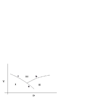
Figure 1: A sketch of the phase diagram for the model, (eq. 1). Phase $I$ correspond to an out-of-plane magnetization, phase $II$ has in-plane magnetization and phase $III$ is paramagnetic. The border line between phase $I$ to phase $II$ is believed to be of first order and from region $I$ and $II$ to $III$ are both second order.

From Monte Carlo (MC) results it is found that there are three regions labelled in the figure 1 as $I,II$ and $III$. Phase $I$ correspond to an out-of-plane magnetization, phase $II$ has in-plane magnetization and phase $III$ is paramagnetic. The border line between phase $I$ to phase $II$ is believed to be of first order and from region $I$ and $II$ to $III$ are both second order.

Although, the different results agree between themselves about the character of the different regions, much care has to be taken because they were obtained by using a cut-off, $r_{c}$, in the dipolar term. The long range character of the potential is lost, consequently we can expect a line of $BKT$ transition coming from region $II$ to region $III$. It is characterized by having no true long range order. This lack of long range order is prevented by the Mermin-Wagner theorem mermin-wagner . The $BKT$ phase transition is an unusual magnetic phase transition characterized by the unbinding of pairs of topological excitations named vortex-anti-vortex berezinskii ; kosterliz-thouless ; teitel ; kogut ; sak ; evaristo1 ; evaristo3 . A vortex (Anti-vortex) is a topological excitation in which spins on a closed path around the excitation core precess by $2\pi$ ($-2\pi$). Above $T_{BKT}$ the correlation length behaves as $\xi\approx\exp(bt^{-1/2})$, with $t\equiv(T-T_{BKT})/T_{BKT}$ and $\xi\rightarrow\infty$ below $T_{BKT}$.

In this work we use MC simulations to investigate the model defined by equation 1. We use a cutoff, $r_{c}$, in the dipolar interaction. Our results strongly suggest that the transition between regions $II$ and $III$ is in the $BKT$ universality class, instead of second order, as found in earlier works.

II Simulation Background

Our simulations are done in a square lattice of volume $L\times L$ ($L=10,20,30,40,50,80$) with periodic boundary conditions. We use the Monte-Carlo method with the Metropolis algorithm evaristo1 ; mc1 ; mc2 ; landau-binder . To treat the dipole term we use a cut-off $r_{c}=5a$, where $a$ is the lattice spacing, as suggested in the work of Santamaria and co-workers santamaria .

We have performed the simulations for temperatures in the range $0.3\leq T\leq 1.2$ at intervals of $\Delta T=0.1$. When necessary this temperature interval is reduced to $\Delta T=0.01$. For every temperature the first $5\times 10^{5}$ MC steps per spin were used to lead the system to equilibrium. The next $10^{6}$ configurations were used to calculate thermal averages of thermodynamical quantities of interest. We have divided these last $10^{6}$ configurations in $20$ bins from which the error bars are estimated from the standard deviation of the averages over these twenty runs. The single-site anisotropy constant was fixed as A = 1.0 while the $D$ parameter was set to $0.10,0.15$ and $0.20$. In this work the energy is measured in units of $JS^{2}$ and temperature in units of $JS^{2}/k_{B}$, where $k_{B}$ is the Boltzmann constant.

To estimate the transition temperatures we use finite-size-scaling (FSS) analysis to the results of our MC simulations. In the following we summarize the main FSS properties. If the reduced temperature is $t=(T-T_{c})/T$, the singular part of the free energy, is given by

$$F(L,T)=L^{-(2-\alpha)/\nu}{\cal F}(tL^{1/\nu})$$ (2)

Appropriate differentiation of $F$ yields the various thermodynamic properties. For an order disorder transition exactly at $T_{c}$ the magnetization, $M$, susceptibility, $\xi$ and specific heat, $C$, behave respectively as landau-binder ; privman .

$$M \propto L^{-\beta/\nu}$$

$$\chi \propto L^{-\gamma/\nu}$$ (3)

$$C \propto L^{-\alpha/\nu}.$$

In addition to these an important quantity is the forth order Binder’s cumulant

$$U_{4}=1-\frac{<m^{4}>}{3<m^{2}>^{2}}.$$ (4)

For large enough $L$, curves for $U_{4}(T)$ cross the same point $U^{*}$ at $T=T_{c}$. For a $BKT$ transition the quantities defined above behave in a different way. Due to the Mermin-Wagner theorem there is no spontaneous magnetization for any finite temperature. The specific heat present a peak at a temperature which is slightly higher than $T_{BKT}$. Beside that, the peak height does not depends on $L$. Because models presenting a $BKT$ transition have an entire critical region, the curves for $U_{4}(L)$ just coincide inside that region presenting no crosses at all. Below we present MC results for three typical regions. When not indicated the error bars are smaller than the symbol sizes.

III Simulation Results

III.1 Case D=0.1

For $D=0.1$ we measured the dependence of the out-of-plane magnetization, $M_{z}$, and the in-plane magnetization , $M_{xy}$, as a function of temperature for several values of $L$ (See figure 2).

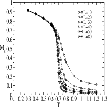
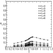
Figure 2: Out-of-plane (left) and in-plane (right) magnetization for $D=0.1$. The ground state is ferromagnetic. There is no in-plane spontaneous magnetization.

The figures indicate that in the ground state the system is aligned in the $z$ direction. Approximately at $T\approx 0.70$ the $M_{z}$ magnetization goes to zero, which gives a rough estimate of the critical temperature. The in-plane magnetization has a small peak close to $T\approx 0.70$. However, the height of the peak diminishes as $L$ grows, in a clear indicative that it is a finite size artifice. The behavior of the specific heat, susceptibility and Binder’s cumulant, are shown in figures 3, 4 and 5 respectively. The results indicate a order-disorder phase transition in clear agreement with references pappas ; allenspach2 ; santamaria ; chui2 .

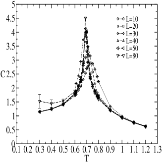
Figure 3: Specific heat as function of temperature for $D=0.1$.

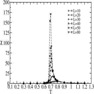
Figure 4: Out-of-plane susceptibility as function of temperature for $D=0.1$.

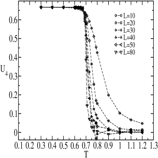
Figure 5: Binder’s cumulant as function of temperature for $D=0.1$.

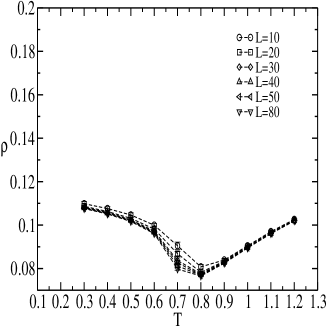
Figure 6: Vortex density in the $xy$ plane for $D=0.1$.

The vortex density in the $xy$ plane (Figure 6) has a very shallow minimum near the estimated critical temperature which is almost independent of the lattice size. The growth of the number of vortices when the temperature is decreased is related to the disordering in the plane when the magnetic moments tend to be in the $z$ direction. We have performed a finite size scaling analysis of the data above by plotting the temperature $T_{c}^{L}$ as a function of $1/L$ for the specific heat, the susceptibility and the crosses of the forth-order cumulant. The results are shown in the table 1. By linear regression we have obtained the critical temperature as $T_{c}^{\infty}=0.682(2)$. An analysis of the behavior of the maxima of the specific heat, $C_{max}$, (See figure 17) as a function of the lattice size shows that it behaves as $C_{max}\propto\ln L$, indicating a second order phase transition. In the phase diagram we crossed the second order line labelled $c$.

L	10	20	30	40	50	80
$C$	0.735	0.711	0.695	0.693	0.690	0.689
$\chi$	0.771	0.729	0.710	0.707	0.700	0.697
$U_{4}$	0.675	0.673	0.673	0.673	0.673	-

Table 1: Critical temperature $T_{c}^{L}$ of the specific heat, $C$, susceptibility, $\chi$, and the crosses of the fourth-order Binder’s cumulante $U_{4}$ as a function of the lattice size $L$. Data are for $D=0.10$

III.2 Case D=0.15

In this region of the parameters, it was observed a transition from an out-of-plane ordering at low temperatures to an in-plane configuration as described by the magnetization behavior shown in Fig. 7. We show $M_{z}$ and $M_{xy}$ in the same figure for comparison. The out-of-plane magnetization goes to zero at $T\approx 0.35$ while an in-plane magnetization sets in. This phenomenon has already been reported experimentally pappas ; allenspach2 and it is due to the competition between the easy axis anisotropy and the dipolar interaction.

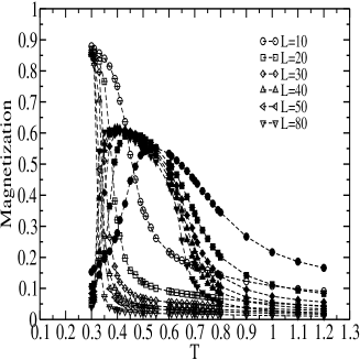
Figure 7: $M_{z}$ and $M_{xy}$ (open and full symbols respectively) for $D=0.15$.

The specific heat curve presents two peaks (See figure 8.). The peak at low temperature is pronounced and is centered in the temperature in which occurs the rapid decrease of the in-plane magnetization, $T_{1}\approx 0.35$. The second peak appears at $T_{2}\approx 0.65$ and seems to be independent of the lattice size.

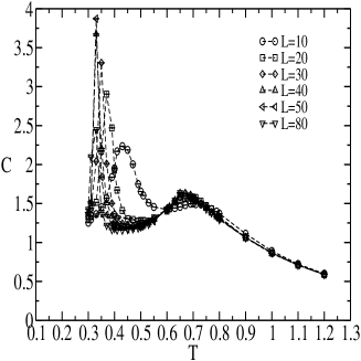
Figure 8: Specific heat for $D=0.15$.

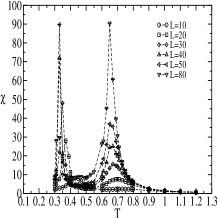
Figure 9: In-plane (left) and out-of-plane (right) susceptibility for $D=0.15$.

In the figure 9 we show the in-plane and out-of-plane susceptibilities. The out-of-plane susceptibility presents a single peak close to $T_{1}\approx 0.35$. The in-plane susceptibility has a maxima at $T_{2}\approx 0.65$ beside the peak at $T_{1}$, indicating two phase transitions. The Binder’s cumulant for the in-plane and out-of-plane magnetization are shown in figures 10. Except for the case $L=10$ the curves for different values of the lattice size do not cross each other indicating a $BKT$ transition at $T\approx T_{2}$. Beside that, the in-plane cumulant has a minimum at $T\approx T_{1}$, which is a characteristic of a first order phase transition landau-binder ; privman .

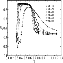
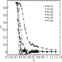
Figure 10: In-plane (left) and out-of-plane (right) Binder’s cumulant as function of temperature for $D=0.15$. Observe that the in-plane cumulant has a minimum at $T\approx 0.35$ indicating a first order phase transition. After the minimum the curves do not cross each other having the same behavior (Except the spurious case $L=10$.) up to $T\approx 0.65$ when they go apart. That is an indication of a $BKT$ phase transition.

The vortex density is shown in figure 11. Its behavior is similar to that one shown in figure 6.

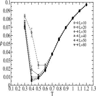
Figure 11: Vortex density as function of temperature for $D=0.15$.

In the phase diagram we crossed the region I to II ($T_{1}$) and II to III ($T_{2}$). The maxima of the specific heat are shown in figure 17 as a function of $L$. It is clear that after a transient behavior it remains constant indicating a $BKT$ transition. A $FSS$ analysis of the susceptibility (see table 2 ) gives the $BKT$ temperature $T_{BKT}^{\infty}=0.613(5)$.

$T_{c}^{L}$	0.729	0.698	0.678	0.670	0.650	0.638
L	10	20	30	40	50	80

Table 2: Critical temperature $T_{c}^{L}$ as a function of the linear size $L$ for the susceptibility $\chi$.

In the phase diagram we crossed the first order line labelled $a$ ($T_{1}$) and the line labelled $b$ ($T_{2}$).

III.3 Case D=0.20

In figure 12 we show the in-plane and out-of-plane magnetization curves for several lattice sizes and $D=0.20$. We observe that as the lattice size $L$ goes from $L=10$ to $L=80$, both magnetization decrease. It can be inferred that as the system approaches the thermodynamic limit, the net magnetization should be zero. Therefore, the system does not present finite magnetization for any temperature $T\neq 0$.

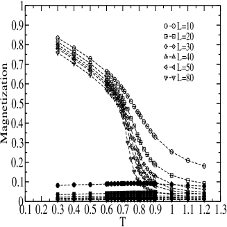
Figure 12: $M_{xy}$ and $M_{z}$ (open and full symbols respectively) for $D=0.2$.

The specific heat (Figure 13) presents a maximum at $T\approx 0.75$. The curves are for different values of $L$. We observe that the position of the maxima and their heights are not affected by the lattice size, all points falling in the same curve.

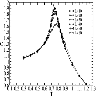
Figure 13: Specific heat for $D=0.2$.The line is a guide to the eyes.

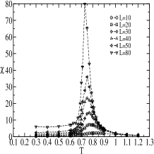
Figure 14: In-plane and out-of-plane susceptibility for $D=0.2$.

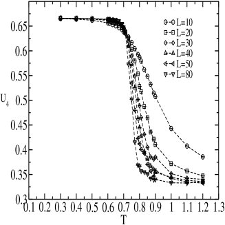
Figure 15: Fourth-order in-plane cumulant for $D=0.2$.

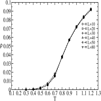
Figure 16: Vortex density in the $xy$ plane for $D=0.2$.

$T_{c}^{L}$	0.829	0.781	0.768	0.753	0.750	0.729
L	10	20	30	40	50	80

Table 3: Critical temperature $T_{c}^{L}$ as a function of the linear size $L$ for the susceptibility $\chi$.

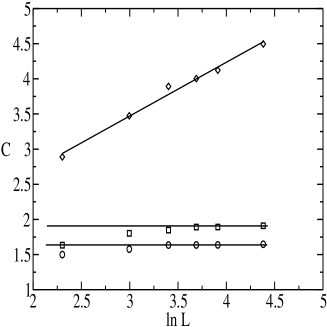
Figure 17: Maxima of the specific heat as a function of the lattice size.

In the figure 14 we show the in-plane and out-of-plane susceptibilities respectively. $\chi^{zz}$ does not present any critical behavior. $\chi^{xy}$ presents a peak which increases with $L$. For the Binder’s cumulant there is no unique cross of the curves. (Except for the $L=10$ curve, which is considered too small to be taken in to account.). This behavior indicates a $BKT$ transition at $T_{BKT}\approx 0.63$. The vortex density, shown in figure 15 is almost independent on the lattice size. In addition, we did a $FSS$ analysis of the susceptibility (see table 3) and the maxima of the specific heat. The specific heat is shown in figure 17. Its behavior indicates a $BKT$ transition. The analysis of the susceptibility gives $T_{BKT}^{\infty}=0.709(5)$. In the phase diagram we crossed the line labelled $b$. In our results we could not detect any other transition for $D=0.20$, indicating that: The line labelled $a$ ends somewhere in between $0.15<D<0.20$ or the crossing at $a$ occurs at a lower temperature ($T<0.30$) outside the range of our simulated data.

IV Conclusions

In earlier studies several authors have claimed that the model for ultrathin magnetic films defined by the equation 1 presents three phases. Referring to figure 1 it is believed that the line labelled $a$ is of first order. The line $b$ and $c$ are of second order. Those results were obtained by introducing a cut off in the long range interaction of the hamiltonian. In the present work we have used a numerical Monte Carlo approach to study the phase diagram of the model for $J=A=1$ and $D=0.10,0.15$ and $0.20$. In order to compare our results to those discussed above we have introduced a cut off in the long range dipolar interaction. A finite size scaling analysis of the magnetization, specific heat, susceptibilities and Binder’s cumulant clearly indicates that the line labelled $a$ is of first order and the line $c$ is of second order in agreement with other results. However, the $b$ line is of $BKT$ type. After analysing the results obtained, some questions come out:

1. Is it possible the existence of a limiting range of interaction in the dipolar term beyond which the character of the transition changes from $BKT$ to second order ?

2. How does the line labelled $a$ end in the phase diagram ?

3. What is the character of the intersection point of the three lines in the phase diagram ?

In a very preliminary calculation Rapini et al.rapini-costa-landau studied the model with true dipolar long range interactions. Their results led them to suspect of a phase transition of the BKT involving the unbinding of vortices-anti-vortices pairs in the model. However, to respond those questions it is necessary to make an more detailed study of the model for several values of the cut off range $r_{c}$. In a simulation program we have to be careful in taking larger $r_{c}$ values since we have to augment the lattice size proportionally to prevent misinterpretations.

V Acknowledgments

Work partially supported by CNPq (Brazilian agency). Numerical work was done in the LINUX parallel cluster at the Laboratório de Simulação Departamento de Física - UFMG.

References

- (1) M.B. Salamon, S. Sinha, J.J. Rhyne, J.E. Cunningham, R.W. Erwin and C.P. Flynn, Phys. Rev. Lett. 56, 259 (1986).
- (2) C.F. Majkrzak, J.M. Cable, J.Kwo, M. Hong, D.B. McWhan, Y. Yafet and C. Vettier, Phys. Rev. Lett. 56, 2700 (1986).
- (3) J.R. Dutcher, B. Heirich, J.F. Cochran, D.A. Steigerwald and W.F. Egelhoff, J. Appl. Phys. 63, 3464 (1988).
- (4) P. Grünberg, R. Schreiber, Y. Pang, M.B. Brodsky and H. Sowers, Phys. Rev. Lett. 57, 2442 (1986).
- (5) F. Saurenbach, U. Walz, L. Hinchey, P. Grünberg and W. Zinn, J. Appl. Phys. 63, 3473 (1988).
- (6) R Allenspach, J. Magn. Magn. Mater. 129, 160 (1994).
- (7) P.M. Lévy, Solid State Phys. 47, 367(1994).
- (8) J.N. Chapman, J. Phys. D 17, 623 (1984).
- (9) A.C. Daykin and J.P. Jakubovics, J. Appl. Phys. 80, 3408 (1986).
- (10) A.B. Johnston, J.N. Chapman, B. Khamsehpour and C.D.W. Wilkinson, J. Phys. D 29, 1419 (1996).
- (11) M. Hehn, J.-P. Boucher, F. Roousseaux, D. Decamini, B. Bartenlian and C. Chappert, Science, 272 1789 (1996).
- (12) S.T. Chui and V.N. Ryzhov, Phys. Rev. Lett. 78, 2224 (1997).
- (13) E.Yu. Vedmedenko, A. Ghazali and J.-C.S. Lévy, Surf. Sci., 402-404, 391 (1998).
- (14) E.Yu. Vedmedenko, A. Ghazali and J.-C.S. Lévy, Phys. Rev. B, 59, 3329 (1999).
- (15) D.P. Pappas, K.P. Kamper and H. Hopster, Phys. Rev. Lett. 64, 3179 (1990).
- (16) R Allenspach and A. Bischof, Phys. Rev. Lett. 69, 3385 (1992).
- (17) C. Santamaria and H.T. Diep, J. Magn. Magn. Mater. 212, 23 (2000).
- (18) M. Rapini, R.A. Dias, D.P. Landau and B. V. Costa, Brasilian Journal of Physics, (2005) (in press).
- (19) S.T. Chui, Phys. Rev. Lett. 74, 3896 (1995).
- (20) Lars Onsager, Phys. Rev. 65,(1944)117.
- (21) M.D. Mermin and H. Wagner, Phys. Rev. Lett. 17, 1133 (1966).
- (22) V.L. Berezinskii, Zh. Eksp. Teo. Fiz. 61, 1144 (1971).
- (23) J.M. Kosterlliz and D.J. Thouless, J. Phys. C 6, 1181 (1973).
- (24) S. Teitel and C. Jayaprakash, Phys. Rev. Lett. 51, 1999 (1983).
- (25) John B. Kogut, Rev. Mod. Phys. 51 (1979)659.
- (26) J. Sak, Phys. Rev. B, 15, 4344 (1977).
- (27) J.E.R. Costa and B.V. Costa, Phys. Rev. B 54,(1996)994.
- (28) J.E.R. Costa, D. P. Landau and B.V.Costa, Phys. Rev. B 57, (1998)11510.
- (29) J. M. Thijssen, Computational Physics, Cambridge University Press (1999).
- (30) S. E. Koonin, D. C. Meredith, Computational Physics, Addisson- Wesley Publishing Company (1990).
- (31) D.P. Landau and K. Binder, A Guide to Monte Carlo Simulations in Statistical Physics (Cambridge University Press, Cambridge).
- (32) V. Privman (ed.), Finite Size Scaling and Numerical Simulation of Statistical Systems (World Scientific, Singapore), 1990.