DSF$-$06/2006
Four variations on Theoretical Physics
by Ettore Majorana

Abstract

An account is given of some topical unpublished work by Ettore Majorana, revealing his very deep intuitions and skilfulness in Theoretical Physics. The relevance of the quite unknown results obtained by him is pointed out as well.

1 Introduction

Probably, the highest appraisal received by the work of Ettore Majorana was expressed by the Nobel Prize Enrico Fermi in several occasions [1], but such opinions could appear as overstatements or unjustified (especially because they are expressed by a great physicist as Fermi), when compared with the spare (known) Majorana’s scientific production, just 9 published papers. However, today the name of Majorana is largely known to the nuclear and subnuclear physicist’s community: Majorana neutrino, Majorana-Heisenberg exchange forces, and so on are, in fact, widely used concepts.

In this paper, we focus on the less-known (or completely unknown) work by this scientist, aimed to shed some light on the peculiar abilities of Majorana that were well recognized by Fermi and his coworkers. The wide unpublished scientific production by Majorana is testified by a large amount of papers [2], almost all deposited at the Domus Galilaeana in Pisa; those known, in Italian, as “Volumetti” has been recently collected and translated in a book [3], and we refer the interested reader to this book for further study.

Here we have chosen to discuss only four topics dealt with by Majorana in different areas of Physics, just to give a sample of his very deep intuitions and skilfulness, together with the relevance of the results obtained.

We start with a discussion of a peculiar approach to Quantum Mechanics, as deduced by a manuscript [4] which probably corresponds to the text for a seminar delivered at the University of Naples in 1938, where Majorana lectured on Theoretical Physics [5]. Some passages of that manuscript reveal a physical interpretation of the Quantum Mechanics, which anticipates of several years the Feynman approach in terms of path integrals, independently of the underlying mathematical formulation. The main topic of that dissertation was the application of Quantum Mechanics to the theory of molecular bonding, but the present scientific interest in it is more centered on the interpretation given by Majorana about some topics of the novel, for that time, Quantum Theory (namely, the concept of quantum state) and the direct application of this theory to a particular case (that is, precisely, the molecular bonding). It not only discloses a peculiar cleverness of the author in treating a pivotal argument of the novel Mechanics, but, keeping in mind that it was written in 1938, also reveals a net advance of at least ten years in the use made of that topic.

In the second topic, we report on a more applicative subject, discussing an original method that leads to a semi-analytical series solution of the Thomas Fermi equation, with appropriate boundary conditions, in terms of only one quadrature [6]. This was developed by Majorana in 1928, just when starting to collaborate (still as a University student) with the Fermi group in Rome, and reveals an outstanding ability to solve very involved mathematical problems in a very interesting and clear way. The whole work performed on the Thomas-Fermi model is contained in some spare sheets, and diligently reported by the author himself in his notebooks [3]. From these it is evident the considerable contribution given by Majorana even in the achievement of the statistical model [7], anticipating, in many respects, some important results reached later by leading specialists. But the major finding by Majorana was his solution (or, rather, methods of solutions) of the Thomas-Fermi equation, which remained completely unknown, until recent times, to the Physics community, who ignored that the non-linear differential equation relevant for atoms and other systems could even be solved semi-analytically. The method proposed by Majorana can also be extended to an entire class of particular differential equations [8].

Afterwards we discuss a subject that was repeatedly studied by Majorana in his research notebooks; namely that of a formulation of Electrodynamics in terms of the electric and magnetic fields, rather than the potentials, which is suitable for a quantum generalization, in a complete analogy with the Dirac theory [9] [10]. This argument was already faced in 1931 by Oppenheimer [11], who only supposed the analogy of the photon case with that described by Dirac, but Majorana explicitly deduced a Dirac-like equation for the photon, thus building up the presumed analogy.

Finally, we report on another topic particularly loved by Majorana, after the appearance (at the end of 1928) of the seminal book by Hermann Weyl [12], that is the Group Theory and its application to physical problem. As testified by the large number of unpublished manuscript pages of the Italian physicist, the Weyl approach greatly influenced the scientific thought and work of Majorana [13]. In fact, when Majorana became aware of the great relevance of the Weyl s application of the Group Theory to Quantum Mechanics, he immediately grabbed the Weyl method and developed it in many applications. In one of his notebooks [3] we find, for example, a preliminary study of what will be one of the most important (published) papers by Majorana on a generalization of the Dirac equation to particles with arbitrary spin [14]. In particular, in 1932 Majorana obtained the infinite-dimensional unitary representations of the Lorentz group that will be re-discovered by Wigner in his 1939 and 1948 works [15], and the entire theory was re-invented by Soviet mathematicians (in particular Gel’fand and collaborators) in a series of articles from 1948 to 1958 [16] and finally applied by physicists years later.

What presented here is, necessarily, a very short account of what Majorana really did in his few years of work (about ten years), but, we hope, it serves in the centennial year at least to understand the very relevant role played by him in the advancement of Physics.

2 Path-Integral approach to Quantum Mechanics

The usual quantum-mechanical description of a given system is strongly centered on the role played by the hamiltonian $H$ of the system and, as a consequence, the time variable plays itself a key role in this description. Such a dissymmetry between space and time variables is, obviously, not satisfactory in the light of the postulates of the Theory of Relativity. This was firstly realized in 1932 by Dirac [17], who put forward the idea of reformulating the whole Quantum Mechanics in terms of lagrangians rather than hamiltonians. The starting point in the Dirac thought is that of exploiting an analogy, holding at the quantum level, with the Hamilton principal function $S$ in Classical Mechanics, thus writing the transition amplitude from one space-time point to another as an (imaginary) exponential of $S$. However, the original Dirac formulation was not free from some unjustified assumptions, leading also to wrong results, and the correct mathematical formulation and the physical interpretation of it came only in the forties with the work by Feynman [18]. In practice, in the Feynman approach to Quantum Mechanics, the transition amplitude between an initial and a final state can be expressed as a sum of the factor ${\mathrm{e}}^{iS[q]/\hbar}$ over all the paths $q$ with fixed end-points, not just those corresponding to classical dynamical trajectories, for which the action is stationary.

In 1938 Majorana was appointed as full professor of Theoretical Physics at the University of Naples, where probably delivered a general conference mentioning also his particular viewpoint on some basic concepts on Quantum Mechanics (see Ref. [4]). Fortunately enough, we have some papers written by him on this subject, and few crucial points, anticipating the Feynman approach to Quantum Mechanics, will be discussed in the following. However, we firstly note that such papers contain nothing of the mathematical aspect of that peculiar approach to Quantum Mechanics, but it is quite evident as well the presence of the physical foundations of it. This is particularly impressive if we take into account that, in the known historical path, the interpretation of the formalism has only followed the mathematical development of the formalism itself.

The starting point in Majorana is to search for a meaningful and clear formulation of the concept of quantum state. And, obviously, in 1938 the dispute is opened with the conceptions of the Old Quantum Theory.

According to the Heisenberg theory, a quantum state corresponds not to a strangely privileged solution of the classical equations but rather to a set of solutions which differ for the initial conditions and even for the energy, i.e. what it is meant as precisely defined energy for the quantum state corresponds to a sort of average over the infinite classical orbits belonging to that state. Thus the quantum states come to be the minimal statistical sets of classical motions, slightly different from each other, accessible to the observations. These minimal statistical sets cannot be further partitioned due to the uncertainty principle, introduced by Heisenberg himself, which forbids the precise simultaneous measurement of the position and the velocity of a particle, that is the determination of its orbit.

Let us note that the “solutions which differ for the initial conditions” correspond, in the Feynman language of 1948, precisely to the different integration paths. In fact, the different initial conditions are, in any case, always referred to the same initial time ($t_{a}$), while the determined quantum state corresponds to a fixed end time ($t_{b}$). The introduced issue of “slightly different classical motions” (the emphasis is given by Majorana himself), according to what specified by the Heisenberg’s uncertainty principle and mentioned just afterwards, is thus evidently related to that of the sufficiently wide integration region required in the Feynman path-integral formula for quantum (rather than classical) systems. In this respect, such a mathematical point is intimately related to a fundamental physical principle.

The crucial point in the Feynman formulation of Quantum Mechanics is, as well-known, to consider not only the paths corresponding to classical trajectories, but all the possible paths joining the initial point with the end one. In the Majorana manuscript, after a discussion on an interesting example on the harmonic oscillator, the author points out:

Obviously the correspondence between quantum states and sets of classical solutions is only approximate, since the equations describing the quantum dynamics are in general independent of the corresponding classical equations, but denote a real modification of the mechanical laws, as well as a constraint on the feasibility of a given observation; however it is better founded than the representation of the quantum states in terms of quantized orbits, and can be usefully employed in qualitative studies.

And, in a later passage, it is more explicitly stated that the wave function “corresponds in Quantum Mechanics to any possible state of the electron”. Such a reference, that only superficially could be interpreted, in the common acceptation, that all the information on the physical systems is contained in the wave function, should instead be considered in the meaning given by Feynman, according to the comprehensive discussion made by Majorana on the concept of state.

Finally we point out that, in the Majorana analysis, a key role is played by the symmetry properties of the physical system.

Under given assumptions, that are verified in the very simple problems which we will consider, we can say that every quantum state possesses all the symmetry properties of the constraints of the system.

The relationship with the path-integral formulation is made as follows. In discussing a given atomic system, Majorana points out how from one quantum state $S$ of the system we can obtain another one $S^{\prime}$ by means of a symmetry operation.

However, differently from what happens in Classical Mechanics for the single solutions of the dynamical equations, in general it is no longer true that $S^{\prime}$ will be distinct from $S$. We can realize this easily by representing $S^{\prime}$ with a set of classical solutions, as seen above; it then suffices that $S$ includes, for any given solution, even the other one obtained from that solution by applying a symmetry property of the motions of the systems, in order that $S^{\prime}$ results to be identical to $S$.

This passage is particularly intriguing if we observe that the issue of the redundant counting in the integration measure in gauge theories, leading to infinite expressions for the transition amplitudes, was raised (and solved) only after much time from the Feynman paper.

3 Solution of the Thomas-Fermi equation

The main idea of the Thomas-Fermi atomic model is that of considering the electrons around the nucleus as a gas of particles, obeying the Pauli exclusion principle, at the absolute zero of temperature. The limiting case of the Fermi statistics for strong degeneracy applies to such a gas. Then, in this approximation, the potential $V$ inside a given atom of charge number $Z$ at a distance $r$ from the nucleus may be written as

$$V(r)=\frac{Ze}{r}\varphi(r).$$ (1)

With a suitable change of variable, $r=\mu x$ and

$$\mu=\frac{1}{2}\left(\frac{3\pi}{4}\right)^{2/3}\frac{\hbar^{2}}{m_{e}e^{2}}Z^{-1/3},$$ (2)

the Thomas-Fermi function $\varphi$ satisfies the following non-linear differential equation (for $\varphi>0$):

$$\varphi^{\prime\prime}=\frac{\varphi^{3/2}}{\sqrt{x}}$$ (3)

(a prime denotes differentiation with respect to $x$) with the boundary conditions:

$$\begin{array}[]{rcl}\varphi(0)&=&1,\\ &&\\ \varphi(\infty)&=&0.\end{array}$$ (4)

The Fermi equation (3) is a universal equation which does not depend neither on $Z$ nor on physical constants ($\hbar,m,e$). Its solution gives, from Eq. (1), as noted by Fermi himself, a screened Coulomb potential which at any point is equal to that produced by an effective charge

$$Ze\,\varphi\left(\frac{r}{\mu}\right).$$ (5)

As was immediately realized, in force of the independence of Eq. (3) on $Z$, the method gives an effective potential which can be easily adapted to describe any atom with a suitable scaling factor, according to Eq. (5).

The problem of the theoretical calculation of observable atomic properties is thus solved, in the Thomas-Fermi approximation, in terms of the function $\varphi(x)$ introduced in Eq. (1) and satisfying the Fermi differential equation (3). By using standard but involved mathematical tools, in his paper [19] Thomas got an exact, “singular” solution of his differential equation satisfying only the second condition (4). This was later (in 1930) considered by Sommerfeld [25] as an approximation of the function $\varphi(x)$ for large $x$ (and is indeed known as the “Sommerfeld solution” of the Fermi equation),

$$\varphi(x)=\frac{144}{x^{3}},$$ (6)

and Sommerfeld himself obtained corrections to the above quantity in order to approximate in a better way the function $\varphi(x)$ for not extremely large values of $x$.

Until recent times it has been believed that the solution of such equation satisfying both the appropriate boundary conditions in (4) cannot be expressed in closed form, and some effort has been made, starting from Thomas [19], Fermi [20], [21] and others, in order to achieve the numerical integration of the differential equation. However, we now know [6], [7] that Majorana in 1927-8 found a semi-analytical solution of the Thomas-Fermi equation by applying a novel exact method [8]. Before proceeding, we will indulge here on an anecdote reported by Rasetti [22], Segrè [23] and Amaldi [24]. According to the last author, “Fermi gave a broad outline of the model and showed some reprints of his recent works on the subject to Majorana, in particular the table showing the numerical values of the so-called Fermi universal potential. Majorana listened with interest and, after having asked for some explanations, left without giving any indication of his thoughts or intentions. The next day, towards the end of the morning, he again came into Fermi’s office and asked him without more ado to draw him the table which he had seen for few moments the day before. Holding this table in his hand, he took from his pocket a piece of paper on which he had worked out a similar table at home in the last twenty-four hours, transforming, as far as Segrè remembers, the second-order Thomas-Fermi non-linear differential equation into a Riccati equation, which he had then integrated numerically.”

The whole work performed by Majorana on the solution of the Fermi equation, is contained in some spare sheets conserved at the Domus Galilaeana in Pisa, and diligently reported by the author himself in his notebooks [3]. The reduction of the Fermi equation to an Abel equation (rather than a Riccati one, as confused by Segrè) proceeds as follows. Let’s adopt a change of variables, from $(x,\varphi)$ to $(t,u)$, where the formula relating the two sets of variables has to be determined in order to satisfy, if possible, both the boundary conditions (4). The function $\varphi$ in Eq. (6) has the correct behavior for large $x$, but the wrong one near $x=0$, so that we could modify the functional form of $\varphi$ to take into account the first condition in (4). An obvious modification is $\varphi=(144/x^{3})f(x)$, with $f(x)$ a suitable function which vanishes for $x\rightarrow 0$ in order to account for $\varphi(x=0)=1$. The simplest choice for $f(x)$ is a polynomial in the novel variable $t$, as it was also considered later, in a similar way, by Sommerfeld [25]. The Majorana choice is as follows:

$$\varphi(x)=\frac{144}{x^{3}}(1-t)^{2},$$ (7)

with $t\rightarrow 1$ as $x\rightarrow 0$. From Eq. (7) we can then obtain the first relation linking $t$ to $x,\varphi$. The second one, involving the dependent variable $u$, is that typical of homogeneous differential equations (like the Fermi equation) for reducing the order of the equation, i.e. exponentiation with an integral of $u(t)$. The transformation relations are thus:

$$\begin{array}[]{rcl}t&=&\displaystyle 1-\frac{1}{12}\sqrt{x^{3}\varphi},\\ &&\\ \varphi&=&e^{\int_{1}^{t}u(t)dt}\,.\end{array}$$ (8)

Substitution into Eq. (3) leads to an Abel equation for $u(t)$,

$$\frac{du}{dt}=\alpha(t)+\beta(t)\,u+\gamma(t)\,u^{2}+\delta(t)\,u^{3},$$ (9)

with

$$\begin{array}[]{rcl}\alpha(t)&=&\displaystyle\frac{16}{3(1-t)},\\ &&\\ \beta(t)&=&\displaystyle 8+\frac{1}{3(1-t)},\\ &&\\ \gamma(t)&=&\displaystyle\frac{7}{3}-4t,\\ &&\\ \delta(t)&=&\displaystyle-\frac{2}{3}t(1-t).\end{array}$$ (10)

Note that both the boundary conditions in (4) are automatically verified by the relations (8). We have reported the derivation of the Abel equation (9) mainly for historical reasons (nevertheless, it is quite important since, in this way, all the theorems on the Abel equation may thus be applied to the non-linear Thomas-Fermi equation too); the precise numerical values for the Fermi function $\varphi(x)$ were obtained by Majorana by solving a different first-order differential equation. Instead of Eq. (7), Majorana chooses $\varphi(x)$ of the form

$$\varphi(x)=\frac{144}{x^{3}}\,t^{6}.$$ (11)

Now the point with $x=0$ corresponds to $t=0$. In order to obtain again a first order differential equation for $u(t)$, the transformation equation for the variable $u$ involves $\varphi$ and its first derivative. Majorana then introduced the following formulas:

$$\begin{array}[]{rcl}t&=&144^{-1/6}\,x^{1/2}\,\varphi^{1/6},\\ &&\\ u&=&\displaystyle-\left(\frac{16}{3}\right)^{1/3}\varphi^{-4/3}\varphi^{\prime}\,\,.\end{array}$$

By taking the $t$-derivative of the last equation in (3) and inserting Eq. (3) in it, one gets:

$$\frac{du}{dt}=-\left(\frac{16}{3}\right)^{1/3}\dot{x}\varphi^{-4/3}\left[-\frac{4}{3}\frac{\varphi^{\prime 2}}{\varphi}+\frac{\varphi^{3/2}}{x^{1/2}}\right].$$ (12)

By using Eqs. (3) to eliminate $x^{1/2}$ and $\varphi^{\prime 2}$, the following equation results:

$$\frac{du}{dt}=\left(\frac{4}{9}\right)^{1/3}\frac{tu^{2}-1}{t}\dot{x}\varphi^{1/3}.$$ (13)

Now the quantity $\dot{x}\varphi^{1/3}$ can be expressed in terms of $t$ and $u$ by making use again of the first equation in (3) (and its $t$-derivative). After some algebra, the final result for the differential equation for $u(t)$ is:

$$\frac{du}{dt}=8\,\frac{tu^{2}-1}{1-t^{2}u}.$$ (14)

The obtained equation is again non-linear but, differently from the original Fermi equation (3), it is first-order in the novel variable $t$ and the degree of non-linearity is lower than that of Eq. (3). The boundary conditions for $u(t)$ are easily taken into account from the second equation in (3) and by requiring that for $x\rightarrow\infty$ the Sommerfeld solution (Eq. (11) with $t=1$) be recovered:

$$\begin{array}[]{rcl}u(0)&=&\displaystyle-\left(\frac{16}{3}\right)^{1/3}\varphi^{\prime}_{0},\\ &&\\ u(1)&=&1.\end{array}$$ (15)

Here we have denoted with $\varphi^{\prime}_{0}=\varphi^{\prime}(x=0)$ the initial slope of the Thomas-Fermi function $\varphi(x)$ which, for a neutral atom, is approximately equal to $-1.588$.

The solution of Eq. (14) was achieved by Majorana in terms of a series expansion in powers of the variable $\tau=1-t$:

$$u=a_{0}+a_{1}\tau+a_{2}\tau^{2}+a_{3}\tau^{3}+...\,\,.$$ (16)

Substitution of Eq. (16) (with the conditions in Eq. (15)) into Eq. (14) results into an iterative formula for the coefficients $a_{n}$ (for details see Ref. [6]). It is remarkable that the series expansion in Eq. (16) is uniformly convergent in the interval $[0,1]$ for $\tau$, since the series $\sum_{n=0}^{\infty}a_{n}$ of the coefficients converges to a finite value determined by the initial slope $\varphi^{\prime}_{0}$. In fact, by setting $\tau=1$ ($t=0$) in Eq. (16) we have from Eq. (15):

$$\sum_{n=0}^{\infty}a_{n}=-\left(\frac{16}{3}\right)\varphi^{\prime}_{0}$$ (17)

Majorana was aware [3] of the fact that the series in Eq. (16) exhibits geometrical convergence with $a_{n}/a_{n-1}\sim 4/5$ for $n\rightarrow\infty$.

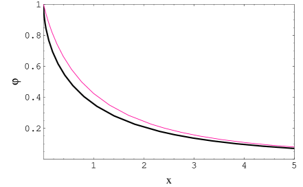
Figure 1: The Thomas-Fermi function $\varphi(x)$ and the Majorana approximation of it. The thin (upper) line refers to the exact (numerical) solution of Eq. (3) while the thick (lower) one corresponds to the parametric solution obtained from Eqs. (19)-(20).

Given the function $u(t)$, we now have to look for the Thomas-Fermi function $\varphi(x)$. This was obtained in a parametric form $x=x(t)$, $\varphi=\varphi(t)$ in terms of the parameter $t$ already introduced in Eq. (3), and by writing $\varphi(t)$ as

$$\varphi(t)=e^{\int_{0}^{t}w(t)dt}$$ (18)

(with this choice, $\varphi(t=0)=1$ and the first condition in (4) is automatically satisfied). Here $w(t)$ is an auxiliary function which is determined in terms of $u(t)$ by substituting Eq. (18) into Eq. (3). As a result, the parametric solution of Eq. (3), with boundary conditions (4), takes the form:

$$\begin{array}[]{rcl}x(t)&=&144^{1/3}\,t^{2}\,e^{2{\cal I}(t)}\\ &&\\ \varphi(t)&=&e^{-6\,{\cal I}(t)}\end{array}$$ (19)

with

$${\cal I}(t)=\int_{0}^{t}\frac{ut}{1-t^{2}u}\,dt$$ (20)

Remarkably, the Majorana solution of the Thomas-Fermi equation is obtained with only one quadrature and gives easily obtainable numerical values for the electrostatic potential inside atoms. By taking into account only $10$ terms in the series expansion for $u(t)$, such numerical values approximate the values of the exact solution of the Thomas-Fermi equation with a relative error of the order of $0.1\%$.

The intriguing property in the Majorana derivation of the solution of the Thomas-Fermi equation is that his method can be easily generalized and may be applied to a large class of particular differential equations, as discussed in [8].

Several generalizations of the Thomas-Fermi method for atoms were proposed as early as in $1928$ by Majorana, but they were considered by the physics community, ignoring the Majorana unpublished works, only many years later.

Indeed, in Sect. 16 of Volumetto II [3], Majorana studied the problem of an atom in a weak external electric field $E$, i.e. atomic polarizability, and obtained an expression for the electric dipole moment for a (neutral or arbitrarily ionized) atom.

Furthermore, he also started to consider the application of the statistical method to molecules, rather than single atoms, studying the case of a diatomic molecule with identical nuclei (see Sect. 12 of Volumetto II [3]). The effective potential in the molecule was cast in the form:

$$V=V_{1}+V_{2}-\alpha\,\frac{2V_{1}V_{2}}{V_{1}+V_{2}},$$ (21)

$V_{1}$ and $V_{2}$ being the potentials generated by each of the two atoms. The function $\alpha$ must obey the differential equation for $V$,

$$\nabla^{2}V=-kV^{3/2}$$ (22)

($k$ is a suitable constant), with appropriate boundary conditions, discussed in [3]. Majorana also gave a general method to determine $V$ when the equipotential surfaces are approximately known (see Sect. 12 of Volumetto III [3]). In fact, writing the approximate expression for the equipotential surfaces, as functions of a parameter $p$, as

$$f(x,y,z)=p,$$ (23)

he deduced a thorough equation from which it is possible to determine $V(\rho)$, when the boundary conditions are assigned. The particular case of a diatomic molecule with identical nuclei was, again, considered by Majorana using elliptic coordinates in order to illustrate his original method [3].

Finally, our author also considered the second approximation for the potential inside the atom, beyond the Thomas-Fermi one, with a generalization of the statistical model of neutral atoms to those ionized $n$ times, including the case $n=0$ (see Sect. 15 of Volumetto II [3]). As recently pointed out, the approach used by Majorana to this end is rather similar to that now adopted in the renormalization of physical quantities in modern gauge theories [26].

4 Majorana formulation of Electrodynamics

In 1931, in his “note on light quanta and the electromagnetic field” [11], Oppenheimer developed an alternative model to the theory of Quantum Electrodynamics, starting from an analogy with the Dirac theory of the electron. Such a formulation was particularly held dear by Majorana, who studied it in some of his unpublished notebooks [9].

Majorana’s original idea was that if the Maxwell theory of electromagnetism has to be viewed as the wave mechanics of the photon, then it must be possible to write the Maxwell equations as a Dirac-like equation for a probability quantum wave $\psi$, this wave function being expressible by means of the physical ${\cal{\vec{E}}}$, ${\cal{\vec{B}}}$ fields. This can be, indeed, realized introducing the quantity

$$\vec{\psi}\;=\;{\cal{\vec{E}}}\;-\;i\,{\cal{\vec{B}}}$$ (24)

since $\vec{\psi}^{\ast}{\cdot}\vec{\psi}\,=\,{\cal{\vec{E}}}^{2}\,+\,{\cal{\vec{B}}}^{2}$ is directly proportional to the probability density function for a photon . In terms of $\vec{\psi}$, the Maxwell equations in vacuum then write

$$\vec{\nabla}{\cdot}\vec{\psi}\;=\;0$$ (25)

$$\frac{\partial\vec{\psi}}{\partial t}\;=\;i\,\vec{\nabla}{\times}\vec{\psi}$$ (26)

By making use of the correspondence principle

$$E \rightarrow i\,\frac{\partial}{\partial t}$$ (27)

$$\vec{p} \rightarrow -i\,\vec{\nabla}$$ (28)

these equations effectively can be cast in a Dirac-like form

$$\left(E\;-\;\alpha{\cdot}\vec{p}\right)\,\vec{\psi}\;=\;0$$ (29)

with the transversality condition

$$\vec{p}{\cdot}\vec{\psi}\;=\;0$$ (30)

where the 3x3 hermitian matrices $(\alpha_{i})_{lm}\,=\,i\,\epsilon_{ilm}$

$$\alpha^{1}\;=\;\left(\begin{array}[]{ccc}0&0&0\\ 0&0&i\\ 0&-i&0\end{array}\right)\;\;\;\;\;\;\;\;\;\;\alpha^{2}\;=\;\left(\begin{array}[]{ccc}0&0&-i\\ 0&0&0\\ i&0&0\end{array}\right)\;\;\;\;\;\;\;\;\;\;\alpha^{3}\;=\;\left(\begin{array}[]{ccc}0&i&0\\ -i&0&0\\ 0&0&0\end{array}\right)$$ (31)

satisfying

$$\left[\alpha_{i}\;,\;\alpha_{j}\right]\;=\;-i\,\epsilon_{ijk}\,\alpha_{k}\\$$ (32)

have been introduced.

The probabilistic interpretation is indeed possible given the “continuity equation” (Poynting theorem)

$$\frac{\partial\rho}{\partial t}\;+\;\vec{\nabla}{\cdot}\vec{j}\;=\;0$$ (33)

where

$$\rho\;=\;\frac{1}{2}\,\vec{\psi}^{\ast}{\cdot}\vec{\psi}\;\;\;\;\;\;\;\;\;\;\;\;\;\;\;\;\vec{j}\;=\;-\,\frac{1}{2}\,\psi^{\ast}\,\alpha\,\psi$$ (34)

are respectively the energy and momentum density of the electromagnetic field.

It is interesting to observe that, differently from Oppenheimer, who started from a mere, presumed analogy with the electron case, Majorana built on analytically the analogy with the Dirac theory, at a dynamical level, by deducing the Dirac-like equation for the photon from the Maxwell equations with the introduction of a complex wave field. As noted by Giannetto in Ref. [10], the Majorana formulation is algebraically equivalent to the standard one of Quantum Electrodynamics and, in addition, also some relevant problems concerning the negative energy states, that induced Oppenheimer to abandon his model, may be elegantly solved by using the method envisaged in a later work [27], thus giving further physical insight into Majorana theory.

5 Lorentz group and its applications

The important role of symmetries in Quantum Mechanics was established in the third decade of the XX century, when it was discovered the special relationships concerning systems of identical particles, reflection and rotational symmetry or translation invariance. Very soon it was discovered that the systematic theory of symmetry resulted to be just a part of the mathematical theory of groups, as pointed out, for example, in the reference book by H. Weil [12]). A particularly intriguing example is that of the Lorentz group which, as well known, underlies the Theory of Relativity, and its representations are especially relevant for the Dirac equation in Relativistic Quantum Mechanics. In the mentioned book, however, although the correspondence between the Dirac equation and the Lorentz transformations is pointed out, the group properties of this connection are not highlighted. Moreover, only a particular kind of such representations are considered (those related to the two-dimensional representations of the group of rotations, according to Pauli), but an exhaustive study of this subject was still lacking at that time.

The situation changes [13] quite sensibly with several (unpublished) papers by Majorana [3], where he gives a detailed deduction of the relationship between the representations of the Lorentz group and the matrices of the (special) unitary group in two dimensions, and a strict connection with the Dirac equation is always taken into account. Moreover the explicit form of the transformations of every bilinear in the spinor field $\Psi$ is reported. For example, Majorana obtains that some of such bilinears behave as the 4-position vector $(ct,x,y,z)$ or as the components of the rank-2 electromagnetic tensor $({\mathbf{E}},{\mathbf{H}})$ under Lorentz transformations, according to the following rules:

$$\Psi^{\dagger}\Psi\sim-i\Psi^{\dagger}\alpha_{x}\alpha_{y}\alpha_{z}\Psi\sim ct,$$

$$-\Psi^{\dagger}\alpha_{x}\Psi\sim i\Psi^{\dagger}\alpha_{y}\alpha_{z}\Psi\sim x,$$

$$-\Psi^{\dagger}\alpha_{y}\Psi\sim i\Psi^{\dagger}\alpha_{z}\alpha_{x}\Psi\sim y,$$

$$-\Psi^{\dagger}\alpha_{z}\Psi\sim i\Psi^{\dagger}\alpha_{x}\alpha_{y}\Psi\sim z,$$

$$i\Psi^{\dagger}\beta\alpha_{x}\Psi\sim E_{x},\quad i\Psi^{\dagger}\beta\alpha_{y}\Psi\sim E_{y},\quad i\Psi^{\dagger}\beta\alpha_{z}\Psi\sim E_{z},$$

$$i\Psi^{\dagger}\beta\alpha_{y}\alpha_{z}\Psi\sim H_{x},\quad i\Psi^{\dagger}\beta\alpha_{z}\alpha_{x}\Psi\sim H_{y},\quad i\Psi^{\dagger}\beta\alpha_{x}\alpha_{y}\Psi\sim H_{z},$$

$$\Psi^{\dagger}\beta\Psi\;\sim\;\Psi^{\dagger}\beta\alpha_{x}\alpha_{y}\alpha_{z}\Psi\;\sim\;1,$$

where $\alpha_{x},\alpha_{y},\alpha_{z},\beta$ are Dirac matrices.

But, probably, the most important result achieved by Majorana on this subject is his discussion of infinite-dimensional unitary representations of the Lorentz group, giving also an explicit form for them. Note that such representations were independently discovered by Wigner in 1939 and 1948 [15] and were thoroughly studied only in the years 1948-1958 [16]. Lucky enough, we are able to reconstruct the reasoning which led Majorana to discuss the infinite-dimensional representations. In Sec. 8 of Volumetto V we read [3]:

“The representations of the Lorentz group are, except for the identity representation, essentially not unitary, i.e., they cannot be converted into unitary representations by some transformation. The reason for this is that the Lorentz group is an open group. However, in contrast to what happens for closed groups, open groups may have irreducible representations (even unitary) in infinite dimensions. In what follows, we shall give two classes of such representations for the Lorentz group, each of them composed of a continuous infinity of unitary representations.”

The two classes of representations correspond to integer and half-integer values for the representation index $j$ (angular momentum). Majorana begins by noting that the group of the real Lorentz transformations acting on the variables $ct,x,y,z$ can be constructed from the infinitesimal transformations associated to the matrices:

$$\begin{array}[]{c}${}$\\ \displaystyle S_{x}\;=\;\left(\begin{array}[]{cccc}0&0&0&0\\ 0&0&0&0\\ 0&0&0&-1\\ 0&0&1&0\end{array}\right),\quad S_{y}\;=\;\left(\begin{array}[]{cccc}0&0&0&0\\ 0&0&0&1\\ 0&0&0&0\\ 0&-1&0&0\end{array}\right),\\ ${}$\\ \displaystyle S_{z}\;=\;\left(\begin{array}[]{cccc}0&0&0&0\\ 0&0&-1&0\\ 0&1&0&0\\ 0&0&0&0\end{array}\right),\\ ${}$\\ \displaystyle T_{x}\;=\;\left(\begin{array}[]{cccc}0&1&0&0\\ 1&0&0&0\\ 0&0&0&0\\ 0&0&0&0\end{array}\right),\quad T_{y}\;=\;\left(\begin{array}[]{cccc}0&0&1&0\\ 0&0&0&0\\ 1&0&0&0\\ 0&0&0&0\end{array}\right),\\ ${}$\\ \displaystyle T_{z}\;=\;\left(\begin{array}[]{cccc}0&0&0&1\\ 0&0&0&0\\ 0&0&0&0\\ 1&0&0&0\end{array}\right),\end{array}$$ (35)

from which he deduces the general commutation relations satisfied by the $S$ and $T$ operators acting on generic (even infinite) tensors or spinors:

$$S_{x}\,S_{y}\,-\,S_{y}\,S_{x} = S_{z},$$

$$T_{x}\,T_{y}\,-\,T_{y}\,T_{x} = -\,S_{z},$$

$$S_{x}\,T_{x}\,-\,T_{x}\,S_{x} = 0,$$ (36)

$$S_{x}\,T_{y}\,-\,T_{y}\,S_{x} = T_{z},$$

$$S_{x}\,T_{z}\,-\,T_{z}\,S_{x} = -\,T_{y},$$

$${\rm{etc}}.$$

Next he introduces the matrices

$$a_{x}\;=\;i\,S_{x},\quad b_{x}\;=\;-i\,T_{x},\quad{\rm{etc.}}$$ (37)

which are Hermitian for unitary representations (and viceversa), and obey the following commutation relations:

$$\left[a_{x},~{}a_{y}\right] = i\,a_{z},$$

$$\left[b_{x},~{}b_{y}\right] = -i\,a_{z},$$

$$\left[a_{x},~{}b_{x}\right] = 0,$$ (38)

$$\left[a_{x},~{}b_{y}\right] = i\,b_{z},$$

$$\left[b_{x},~{}a_{y}\right] = i\,b_{z},$$

$${\rm{etc}}.$$

By using only these relations he then obtains (algebraically ) the explicit expressions of the matrix elements for given $j$ and $m$ [3] [14]. The non-zero elements of the infinite matrices $a$ and $b$, whose diagonal elements are labelled by $j$ and $m$, are as follows:

$$\!\!\!\!\!\displaystyle<j,m\,|\,a_{x}-ia_{y}\,|\,j,m+1> = \displaystyle\sqrt{(j+m+1)(j-m)},$$

$$\!\!\!\!\!\displaystyle<j,m\,|\,a_{x}+ia_{y}\,|\,j,m-1> = \displaystyle\sqrt{(j+m)(j-m+1)},$$

$$\!\!\!\!\!\displaystyle<j,m\,|\,a_{z}\,|\,j,m> = \displaystyle m,$$

$$\!\!\!\!\!\displaystyle<j,m\,|\,b_{x}-ib_{y}\,|\,j+1,m+1> = \displaystyle-\,\frac{1}{2}\,\sqrt{(j+m+1)(j+m+2)},$$

$$\!\!\!\!\!\displaystyle<j,m\,|\,b_{x}-ib_{y}\,|\,j-1,m+1> = \displaystyle\frac{1}{2}\,\sqrt{(j-m)(j-m-1)},$$ (39)

$$\!\!\!\!\!\displaystyle<j,m\,|\,b_{x}+ib_{y}\,|\,j+1,m-1> = \displaystyle\frac{1}{2}\,\sqrt{(j-m+1)(j-m+2)},$$

$$\!\!\!\!\!\displaystyle<j,m\,|\,b_{x}+ib_{y}\,|\,j-1,m-1> = \displaystyle-\,\frac{1}{2}\,\sqrt{(j+m)(j+m-1)},$$

$$\!\!\!\!\!\displaystyle<j,m\,|\,b_{z}\,|\,j+1,m> = \displaystyle\frac{1}{2}\,\sqrt{(j+m+1)(j-m+1)},$$

$$\!\!\!\!\!\displaystyle<j,m\,|\,b_{z}\,|\,j-1,m> = \displaystyle\frac{1}{2}\,\sqrt{(j+m)(j-m)}.$$

The quantities on which $a$ and $b$ act are infinite tensors or spinors (for integer or half-integer $j$, respectively) in the given representation, so that Majorana effectively constructs, for the first time, infinite-dimensional representations of the Lorentz group. In [14] the author also picks out a physical realization for the matrices $a$ and $b$ for Dirac particles with energy operator $H$, momentum operator $\mathbf{p}$ and spin operator $\mathbf{\sigma}$:

$$a_{x}\,=\,\frac{1}{\hbar}\left(yp_{z}-zp_{y}\right)+\frac{1}{2}\sigma_{x},\quad b_{x}\,=\,\frac{1}{\hbar}x\frac{H}{c}+\frac{i}{2}\alpha_{x},\quad{\rm{etc.}},$$ (40)

where $\alpha_{x},\alpha_{y},\alpha_{z}$ are the Dirac $\alpha$-matrices.

Further development of this material then brought Majorana to obtain a relativistic equation for a wave-function $\psi$ with infinite components, able to describe particles with arbitrary spin (the result was published in 1932 [14]). By starting from the following variational principle:

$$\delta\int\overline{\psi}\left(\frac{H}{c}+{\mathbf{\alpha}}\cdot{\mathbf{p}}-\beta mc\right)\psi\,d^{4}x\,=\,0,$$ (41)

By requiring the relativistic invariance of the variational principle in Eq. (41), Majorana deduces both the transformation law for $\psi$ under an (infinitesimal) Lorentz transformation and the explicit expressions for the matrices ${\mathbf{\alpha}}$, $\beta$. In particular, the transformation law for $\psi$ is obtained directly from the corresponding ones for the variables $ct,x,y,z$ by means of the matrices $a$ and $b$ in the representation (40). By using the same procedure leading to the matrix elements in (39), Majorana gets the following expressions for the elements of the (infinite) Dirac $\mathbf{\alpha}$ and $\beta$ matrices:

$$\!\!\!\!\!\displaystyle<j,m\,|\,\alpha_{x}-i\alpha_{y}\,|\,j+1,m+1> = \displaystyle-\,1/2\,\sqrt{\frac{(j+m+1)(j+m+2)}{\displaystyle\left(j+1/2\right)\left(j+3/2\right)}},$$

$$\!\!\!\!\!\displaystyle<j,m\,|\,\alpha_{x}-i\alpha_{y}\,|\,j-1,m+1> = \displaystyle-\,1/2\,\sqrt{\frac{(j-m)(j-m-1)}{\displaystyle\left(j-1/2\right)\left(j+1/2\right)}},$$

$$\!\!\!\!\!\displaystyle<j,m\,|\,\alpha_{x}+i\alpha_{y}\,|\,j+1,m-1> = \displaystyle 1/2\,\sqrt{\frac{(j-m+1)(j-m+2)}{\displaystyle\left(j+1/2\right)\left(j+3/2\right)}},$$

$$\!\!\!\!\!\displaystyle<j,m\,|\,\alpha_{x}+i\alpha_{y}\,|\,j-1,m-1> = \displaystyle 1/2\,\sqrt{\frac{(j+m)(j+m-1)}{\displaystyle\left(j-1/2\right)\left(j+1/2\right)}},$$ (42)

$$\!\!\!\!\!\displaystyle<j,m\,|\,\alpha_{z}\,|\,j+1,m> = \displaystyle-\,1/2\,\sqrt{\frac{(j+m+1)(j-m+1)}{\displaystyle\left(j+1/2\right)\left(j+3/2\right)}},$$

$$\!\!\!\!\!\displaystyle<j,m\,|\,\alpha_{z}\,|\,j-1,m> = \displaystyle-\,1/2\,\sqrt{\frac{(j+m)(j-m)}{\displaystyle\left(j-1/2\right)\left(j+1/2\right)}},$$

$$\!\!\!\!\!\displaystyle\beta = \frac{1}{\displaystyle j+1/2}.$$

The Majorana equation for particles with arbitrary spin has, then, the same form of the Dirac equation:

$$\left(\frac{H}{c}+{\mathbf{\alpha}}\cdot{\mathbf{p}}-\beta mc\right)\psi\,=\,0,$$ (43)

but with different (and infinite) matrices $\alpha$ and $\beta$, whose elements are given in Eqs. (42). The rest energy of the particles thus described has the form:

$$E_{0}\,=\,\frac{mc^{2}}{\displaystyle s+1/2},$$ (44)

and depends on the spin $s$ of the particle. We here stress that the scientific community of that time was convinced that only equations of motion for spin 0 (Klein-Gordon equation) and spin 1/2 (Dirac equation) particles could be written down. The importance of the Majorana work was first realized by van der Waerden [29] but, unfortunately, the paper remained unnoticed until recent times.

Acknowledgments

The author warmly thanks I. Licata for his kind spur to write the present paper and E. Recami for fruitful discussions.

References

- [1] See the contribution by E. Recami in this volume.
- [2] The list of the unpublished scientific Manuscript by Majorana can be found in E. Recami, Quaderni di Storia della Fisica, 5 (1999) 19.
- [3] S. Esposito, E. Majorana jr, A. van der Merwe and E. Recami (eds.) Ettore Majorana: Notes on Theoretical Physics (Kluwer, New York, 2003).
- [4] S. Esposito, Quaderni di Storia della Fisica, to be published; arXiv:physics/0512174.
- [5] E. Majorana, Lezioni all’Università di Napoli, (Bibliopolis, Napoli, 1987). E. Majorana, Lezioni di Fisica Teorica, edited by S. Esposito (Bibliopolis, Napoli, 2006) (in press). S. Esposito, Il Nuovo Saggiatore, 21 (2005) 21; A. Drago and S. Esposito, e-print arXiv:physics/0503084.
- [6] S. Esposito, Am. J. Phys. 70 (2002) 852; arXiv:physics/0111167.
- [7] E. Di Grezia and S. Esposito, Found. Phys. 34 (2004) 1431; e-print arXiv:physics/0406030.
- [8] S. Esposito, Int. J. Theor. Phys. 41 (2002) 2417; e-print arXiv:math-ph/0204040.
- [9] R. Mignani, E. Recami and M. Baldo, Lett. Nuovo Cim. 11 (1974) 568; see also E. Giannetto, Lett. Nuovo Cim. 44 (1985) 140 and 145. S. Esposito, Found. Phys. 28 (1998) 231; e-print arXiv:hep-th/9704144.
- [10] E. Giannetto, in F. Bevilacqua (ed.) Atti IX Congresso Naz.le di Storia della Fisica (Milan, 1988) p.173.
- [11] J.R. Oppenheimer, Phys. Rev. 38 (1931) 725.
- [12] H. Weyl, Gruppentheorie und Quantenmechanik, first edition (Hirzel, Leipzig, 1928); English translation from the second German edition in The Theory of Groups and Quantum Mechanics (Dover, New York 1931).
- [13] A. Drago and S. Esposito, Found. Phys. 34 (2004) 871; arXiv:physics/0503084.
- [14] E. Majorana, Nuovo Cim. 9 (1932) 335.
- [15] E. Wigner, Ann. Math. 40 (1939) 149.
- [16] I.M. Gel’fand, A.M. Yaglom, Zh. Ehksp. Teor. Fiz. 18 (1948) 703; I.M. Gel’fand, R.A. Minlos, Z.Ya. Shapiro, Representations of the Rotation and Lorentz Groups and their Applications (Pergamon Press, Oxford, 1963).
- [17] P. A. M. Dirac, Phys. Zeits. Sowjetunion 3 (1933) 64.
- [18] R. P. Feynman, The Principle of Least Action in Quantum Mechanics (Princeton University, Ann Arbor, 1942; University Microfilms Publication No. 2948). R. P. Feynman, Rev. Mod. Phys. 20 (1948) 367.
- [19] L.H. Thomas, Proc. Camb. Phil. Soc. 23 (1926) 542.
- [20] E. Fermi, Rend. Lincei 6 (1927) 602.
- [21] E. Fermi, Falkenhagen, Quantentheorie und Chemie, Leipziger Vortraege 95 (1928).
- [22] F. Rasetti in E. Fermi Collected Papers (Note e Memorie) (University of Chicago Press, Chicago, 1962) p. 277.
- [23] E. Segré, A Mind Always in Motion (University of California Press, Berkeley, 1993).
- [24] E. Amaldi, Ettore Majorana: Man and Scientist, in A. Zichichi (ed.) Strong and Weak Interactions. Present problems (Academic Press, New York, 1966).
- [25] A. Sommerfeld, Rend. Lincei 15 (1932) 788.
- [26] S. Esposito, preprint arXiv:physics/0512259.
- [27] E. Majorana, Nuovo Cim. 14 (1937) 171.
- [28] J.J. Sakurai, Modern Quantum Mechanics (Benjamin-Cummings, Menlo Park, 1985).
- [29] Letter from Leipzig by Ettore Majorana to his father dated February 18, 1933, quoted by Recami in Ettore Majorana, Lezioni all’Università di Napoli in [5].