Recurrent motions within plane Couette turbulence

Abstract

The phenomenon of bursting, in which streaks in turbulent boundary layers oscillate and then eject low speed fluid away from the wall, has been studied experimentally, theoretically, and computationally for more than 50 years because of its importance to the three-dimensional structure of turbulent boundary layers. We produce five new three-dimensional solutions of turbulent plane Couette flow, one of which is periodic while four others are relative periodic. Each of these five solutions demonstrates the break-up and re-formation of near-wall coherent structures. Four of our solutions are periodic but with drifts in the streamwise direction. More surprisingly, two of our solutions are periodic but with drifts in the spanwise direction, a possibility that does not seem to have been considered in the literature. We argue that a considerable part of the streakiness observed experimentally in the near-wall region could be due to spanwise drifts that accompany the break-up and re-formation of coherent structures. We also compute a new periodic solution of plane Couette flow that could be related to transition to turbulence.

The violent nature of the bursting phenomenon implies the need for good resolution in the computation of periodic and relative periodic solutions within turbulent shear flows. We address this computationally demanding requirement with a new algorithm for computing relative periodic solutions one of whose features is a combination of two well-known ideas — namely the Newton-Krylov iteration and the locally constrained optimal hook step. Each of our six solutions is accompanied by an error estimate.

In the concluding discussion, we discuss dynamical principles that suggest that the bursting phenomenon, and more generally fluid turbulence, can be understood in terms of periodic and relative periodic solutions of the Navier-Stokes equation.

1 Introduction

Turbulent boundary layers are characterized by a viscous sublayer, in which the mean streamwise velocity nearly equals the distance from the wall in wall units, a buffer layer, and a logarithmic boundary layer. The impressive agreement of theoretical predictions of the mean streamwise velocity in the viscous sublayer and the logarithmic boundary layer with experiment (Monin and Yaglom, 1971, p. 273) and with computation (Kim et al., 1987) can be considered an outstanding success in the effort to understand turbulence in fluid flows. It was initially believed that the flow in the viscous sublayer was laminar, but experiments in the 50s and 60s lead to the conclusion that random fluctuations exist in this layer even though the mean streamwise velocity in this layer had a laminar profile (Monin and Yaglom, 1971, p. 270).

The phenomenon of bursting became evident during investigations of the viscous sublayer and the buffer region (Kline et al., 1967; Klebanoff et al., 1962). In this phenomenon, streaks in the near-wall region break-up and re-form in a quite striking manner. Much of the turbulent energy production occurs in the buffer and viscous layers (Kline et al., 1967) and the three-dimensional structure of turbulent boundary layers appears to be intimately related to bursting. Because of this connection and because of the striking nature of the phenomenon itself, bursting has been the subject of numerous experimental (Acarlar and Smith, 1987; Bech et al., 1995; Kline et al., 1967; Klebanoff et al., 1962; Smith and Metzler, 1983) and computational or theoretical studies (Hamilton et al., 1995; Holmes et al., 1996; Itano and Toh, 2001, 2005; Jiménez et al., 2005; Kawahara and Kida, 2001; Schoppa and Hussain, 2002). There has been some discussion in the literature of exactly what is meant by bursting (Itano and Toh, 2001; Jiménez et al., 2005). In this paper, bursting will always refer to the break-up and re-formation of coherent structures, such as streaks, in turbulent buffer regions.

Although bursting has been much studied, its dynamics has proved elusive. A large number of mechanisms have been proposed to explain bursting (Hamilton et al., 1995; Itano and Toh, 2001; Kline et al., 1967; Klebanoff et al., 1962; Schoppa and Hussain, 2002). The word mechanism in this context does not refer to new physical principles. There is no doubt at all that the incompressible Navier-Stokes equation is adequate to explain the dynamics of bursting, and the physics of bursting is the physics that goes into that equation and its boundary conditions. However, as is well known, the nature of the solutions of the Navier-Stokes equation in the turbulent regime is poorly understood. These mechanisms try to provide a way to approximately understand some solutions of the Navier-Stokes equation.

Although approximate, some mechanisms can be useful for computing exact solutions as shown by the construction of traveling wave and steady solutions of channel flows by Waleffe (Waleffe, 1998, 2001, 2003). The method introduced in that body of work was later adapted to pipe flows (Faisst and Eckhardt, 2003; Wedin and Kerswell, 2004). However, the break-up and re-formation of coherent structures cannot be studied using traveling waves or steady solutions.

It is certainly very desirable to find exact solutions of the Navier-Stokes equation that correspond to bursting. These solutions will provide a solid and reliable route to understanding the dynamics of bursting. In this context, it is noteworthy that the self-sustaining process mechanism indeed suggested the existence of periodic solutions that correspond to bursting (Hamilton et al., 1995; Kawahara and Kida, 2001; Waleffe, 1997). We follow Hamilton et al. (1995) and conduct our computations using plane Couette flow at a Reynolds number ($Re$) of 400. In plane Couette flow two parallel walls move in opposite directions with equal speed and drive the fluid in-between. The Reynolds number is based on half the separation between the walls and half the difference between the wall velocities. To render the computational domain finite, we assume the domain to be periodic in the streamwise and spanwise directions, with periods equal to $2\pi\Lambda_{x}$ and $2\pi\Lambda_{z}$. Unless otherwise stated, our computations use $\Lambda_{x}=0.875$ and $\Lambda_{z}=0.6$ to facilitate comparison with earlier computations and because of particular advantages of this box described in (Hamilton et al., 1995). The walls are assumed to be at $y=\pm 1$, with the upper wall moving in the $x$ or streamwise direction in the positive sense with speed equal to $1$.

It is known experimentally that the details of bursting in the near-wall region are remarkably similar over a very wide range of Reynolds numbers (Smith and Metzler, 1983). Thus our use of $Re=400$ in plane Couette flow is an acceptable choice. Turbulent spots have been observed in plane Couette flow experiments at $Re=360$ (Bech et al., 1995).

Marker	Label	$s_{x}/2\pi\Lambda_{x}$	$s_{z}/2\pi\Lambda_{z}$	$T/T^{+}$	$\lambda_{max}$	$Re_{\tau}$	$(2L,M,2N)$	error
$\ast$	$P_{1}$	$0$	$0$	$82.7$/$167$	$24.5$	$56.9$	$(32,64,48)$	$10^{-7}$
o	$P_{2}$	$.15$	$-.28$	$70.9$/$197$	$12.2$	$66.3$	$(48,64,48)$	$10^{-5}$
$\Box$	$P_{3}$	$.03$	$0$	$77.1$/$216$	$4.4+\iota 3.6$	$66.9$	$(64,56,48)$	$10^{-5}$
$\Diamond$	$P_{4}$	$.01$	$.08$	$102.7$/$287$	$5.1+\iota 16.4$	$66.8$	$(48,48,32)$	$10^{-3}$
$\triangle$	$P_{5}$	$.22$	$0$	$91$/$266$	$-11.5$	$68.4$	$(48,64,48)$	$10^{-4}$
$\nabla$	$P_{6}$	$0$	$0$	$87.9$/$259$	$-14.6$	$68.6$	$(48,64,48)$	$10^{-5}$

Table 1: This table gives data for six periodic and relative periodic solutions of plane Couette flow labeled $P_{1}$ through $P_{6}$. The markers in the first column are used to distinguish between these solutions in later plots. The shifts $s_{x}$ and $s_{z}$ are explained in the text. The $T/T^{+}$ column gives the period, with $T^{+}$ being the period in wall units. The $\lambda_{max}$ column gives the maximum characteristic multiplier. The last three columns report the frictional Reynolds number, the resolution of the computational grid, and the relative error in the computation.

Table 1 reports data for six periodic or relative periodic solutions that we computed. The final velocity field obtained by integrating the initial velocity field over one full period equals the initial velocity field for periodic solutions. But for relative periodic solutions the final velocity field equals the initial velocity field after shifts equal to $s_{x}$ and $s_{z}$ in the streamwise and spanwise directions, respectively. These shifts, which are reported in Table 1, are both $0$ for $P_{1}$ and $P_{6}$. Thus both those solutions are periodic. The equations of plane Couette flow are unchanged by translations in the streamwise and spanwise directions. The existence of relative periodic solutions is possible because of those invariances.

Frictional velocity and frictional length can be obtained using the mean shear at the wall (Monin and Yaglom, 1971, p. 265). Those quantities are the basis of wall units. Throughout this paper, wherever wall units are used, the mean shear is obtained by averaging at the upper wall over one single period of a periodic or relative periodic solution. Following standard practice, the use of wall units is signaled by using $+$ as a superscript. The frictional Reynolds number $Re_{\tau}$ was obtained using the mean shear at the upper wall and the distance between the two walls. Table 1 shows that the $Re_{\tau}$ for $P_{1}$ is significantly lower than it is for the other solutions. This is because $P_{1}$ alone is related to transition to turbulence, while all the others are related to bursting.

Kawahara and Kida (2001) found a periodic solution of plane Couette flow with period equal to $85.5$ which appears similar to $P_{1}$. However, their solution satisfies the shift-reflection and shift-rotation symmetries of plane Couette flow (Kawahara, 2005). Although $P_{1}$ has zero mass flux in the streamwise direction like their solution, it is very far from satisfying either symmetry as will be shown. Therefore $P_{1}$ is a new solution. The bursting solutions $P_{2}$ through $P_{6}$ are all new, and we will presently argue that these are the first computations of bursting periodic or relative periodic solutions that demonstrably correspond to solutions of the Navier-Stokes equation.

All the characteristic multipliers $\lambda_{max}$ listed in Table 1 are outside the unit circle, which implies instability of the solutions $P_{1}$ through $P_{6}$. Yet we report relative errors for all these solutions. A relative error of $10^{-7}$ implies that the computed solution matches a solution of the Navier-Stokes equation up to at least $7$ digits. The manner in which these error estimates were found is explained in Section 3. Significantly, these error estimates can be verified using any good DNS (direct numerical simulation) code in spite of the instability of the underlying solutions. Such quantitative reproducibility is a step forward for turbulence computations.

The numbers $2L$, $M$, and $2N$ in Table 1 give the number of grid points in the $x$, $y$, and $z$ directions. We used a Fourier grid in the $x$ and $z$ directions and a Chebyshev grid in the $y$ direction. Good spatial resolution is the key to finding solutions that are not numerical artifacts. Hamilton et al. (1995) and Kawahara and Kida (2001) used $(2L,M,2N)=(16,32,16)$ in their plane Couette flow computations. The evidence for striking recurrences and the existence of periodic solutions offered in these works is significant. However, estimates for spatial discretization error described in Section 3 imply that the spatial discretization error with $(2L,M,2N)=(16,32,16)$ for bursting solutions is at least $5\%$ and can be twice as much.

A section 2, we describe a new method for finding periodic and relative periodic solutions. The number of degrees of freedom that determine the initial velocity field for $P_{3}$ is $319790$ and the number of degrees of freedom for $P_{2}$, $P_{5}$, and $P_{6}$ is $273918$. These numbers exceed the number of degrees of freedom in any earlier computation of periodic solutions by at least a factor of $20$, and our method can also compute relative periodic solutions. One feature of the method is a combination of the Newton-Krylov iteration (Kelley, 2003; Sancheź et al., 2004) with the locally constrained optimal hook step (Dennis and Schnabel, 1996). The locally constrained optimal hook step is related to the Levenberg-Marquardt procedure and is a well-established idea in optimization. However, its possibilities seem to have been largely overlooked in computations of periodic and steady solutions. The combination of Newton-Krylov iterations with the locally constrained optimal hook step is simple, but powerful. It is much more effective than the often used damped Newton iteration.

In Section 4, we develop the connection of the computations summarized in Table 1 to the dynamics of the bursting phenomenon. There has been some discussion about whether the near-wall bursting observed experimentally is due to the advection of coherent objects or to the break-up and re-formation of coherent objects (Jiménez et al., 2005). The relative periodic solutions reported in Table 1, and especially the spanwise drifts of $P_{2}$ and $P_{4}$, will be shown to be significant in this respect.

In the concluding Section 5, we discuss our belief that a good route to understanding the dynamics of a differential equation is by computing its solutions and recognizing the relationship between those solutions. We discuss dynamical principles that suggest that infinitely many periodic and relative periodic motions can be found within turbulent flows. About half a century ago, a common belief was that linearly stable solutions are observed in nature and in experiment, while the unstable ones are not. Although all these infinitely many periodic and relative periodic motions are certain to be linearly unstable, their instability is only a manifestation of the instability of turbulent flows. In spite of their instability, these solutions are relevant both to natural phenomena and experiment as we demonstrate in Section 4 and as we argue in Section 5.

The idea of understanding phenomena using well-resolved and linearly unstable nonlinear solutions is beginning to take root in recent research on the transition to turbulence in shear flows (Kerswell, 2005). Linearly unstable nonlinear traveling waves have been observed in a pipe flow experiment (Hof et al., 2004). Although transition to turbulence in pipe and channel flows is still an unsolved problem, there can be little doubt that the nonlinear traveling waves such as the ones observed by Hof et al. (2004) will be an important part of an eventual solution of the transition problem. Periodic and relative periodic solutions are the next step for understanding turbulent phenomena such as bursting.

2 A numerical method for finding relative periodic solutions

This section describes a numerical method for finding periodic and relative periodic solutions in plane Couette flow. Although the description of the numerical method is specific to plane Couette flow, it can be easily adapted to other partial differential equations. Our method has three new aspects. Firstly, we describe a way to find good initial guesses. Secondly, we show how to set up the Newton equations for finding relative periodic solutions. Thirdly, we show how to modify the Newton-Krylov procedure to compute the locally constrained optimal hook step.

The Navier-Stokes equation for incompressible flow takes the form

$$\partial{\bf u}/\partial t+({\bf u}.\nabla){\bf u}=-(1/\rho)\nabla p+(1/Re)\triangle{\bf u}$$ (2.1)

with the incompressibility constraint implying $\nabla.{\bf u}=0$. For plane Couette flow, the boundary conditions are ${\bf u}=(\pm 1,0,0)$ at the walls (which are at $y=\pm 1$) in the $y$ or wall-normal direction, and periodic in the other two directions with periods equal to $2\pi\Lambda_{x}$ and $2\pi\Lambda_{z}$. The equation cannot be viewed as a dynamical system when written in this form because the velocity field ${\bf u}$ has to satisfy the zero divergence condition and there is no explicit equation for evolving the pressure $p$ in time. It is necessary to rewrite the equation as a dynamical system for the purpose of computing periodic and relative periodic solutions.

The pressure term can be completely eliminated by recasting (2.1) in terms of the wall-normal velocity $v(x,y,z)$, the wall-normal vorticity $\eta(x,y,z)$, and the mean components $\bar{u}(y)$ and $\bar{w}(y)$ of the streamwise and spanwise velocities. The boundary conditions become $\bar{u}(\pm 1)=\pm 1$, $\bar{w}(\pm 1)=0$, and $v(x,\pm 1,z)=v_{y}(x,\pm 1,z)=\eta(x,\pm 1,z)=0$. The velocity field ${\bf u}$ can be constructed from $\bar{u}$, $\bar{w}$, $v$, and $\eta$ using $\nabla.{\bf u}=0$. The velocity component $v$ and the vorticity component $\eta$ are discretized in the $x$ and $z$ directions using Fourier modes. For example,

$$v(x,y,z)=\sum_{\begin{subarray}{c}-L<l<L\\ -N<n<N\end{subarray}}\hat{v}_{l,n}(y)\exp\Bigl{(}\frac{\iota lx}{\Lambda_{x}}+\frac{\iota nz}{\Lambda_{z}}\Bigr{)},$$ (2.2)

where the dependence on $t$ is not shown explicitly. The Fourier modes $\hat{\eta}_{l,n}$ are defined by replacing $v$ by $\eta$ in (2.2).

Kim et al. (1987) proposed a very good numerical method for integrating the Navier-Stokes equation using this formulation and we follow their approach. The Navier-Stokes equation (2.1) becomes a dynamical system in this formulation.

We use a Fourier grid with $2L$ and $2N$ points in the $x$ and $z$ directions, but we always set the modes with $l=L$ or $n=N$ equal to $0$. We use $M+1$ Chebyshev points in the $y$ direction. After spatial discretization, the dynamical system has approximately $8LMN$ degrees of a freedom. A count that takes into account the boundary conditions on $\bar{u}$, $\bar{w}$, $v$ and $\eta$, the treatment of modes with $l=L$ or $n=N$, and the fact that the mean components of $v$ and $\eta$ are always zero gives $2(M-1)+(2M-4)((2N-1)(2L-1)-1)$ as the exact number of degrees of freedom. It is important to get the number of degrees of freedom exactly right. The spatially discretized system can be thought of as a dynamical system of the form $\dot{X}=f(X)$, where the $2(M-1)+(2M-4)((2N-1)(2L-1)-1)$ components of $X$ encode $\bar{u}$, $\bar{w}$, $v$ and $\eta$. All the components of $X$ are real numbers.

Our code implements the nonlinear terms in advection, rotation, and skew-symmetric forms. The viscous terms are treated implicitly and the advection terms are treated explicitly when discretizing time. The code employs dealiasing using the $3/2$ rule in the $x$ and $z$ directions. The code was tested using three-dimensional modes of the Orr-Sommerfeld equation and in various other ways.

2.1 Finding initial guesses

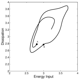
Figure 1: This figure shows the projection of a trajectory of plane Couette flow onto the energy dissipation ($D$) and energy input($I$) plane

To find an initial guess for a relative periodic solution, we begin by looking at projections of trajectories to the energy dissipation and energy input plane. The rate of energy dissipation per unit volume for plane Couette flow is given by

$$D=\frac{1}{8\pi^{2}\Lambda_{x}\Lambda_{z}}\int_{0}^{2\pi\Lambda_{z}}\int_{-1}^{+1}\int_{0}^{2\pi\Lambda_{x}}\left|\nabla u\right|^{2}+\left|\nabla v\right|^{2}+\left|\nabla w\right|^{2}\>dx\,dy\,dz$$ (2.3)

and the rate of energy input per unit volume is given by

$$I=\frac{1}{8\pi^{2}\Lambda_{x}\Lambda_{z}}\int_{0}^{2\pi\Lambda_{x}}\int_{0}^{2\pi\Lambda_{z}}\frac{\partial u}{\partial y}\Bigl{\lvert}_{y=1}+\frac{\partial u}{\partial y}\Bigl{\lvert}_{y=-1}\>dx\,dz.$$ (2.4)

For the laminar solution $(u,v,w)=(y,0,0)$, both $D$ and $I$ are normalized to evaluate to $1$.

The trajectory that starts at $A$ in Figure 1 appears to come close at $B$. But that close approach is not significant because even distant points in phase space can coincide in a two-dimensional projection. What we look for is the resemblance of the shape of the trajectory from $B$ onwards with the shape of the trajectory from $A$ onwards. In Figure 1, the trajectory that begins at $A$ develops a type of protrusion in the upper right part of the figure, but the trajectory that begins at $B$ does not. Therefore, $A$ would not be a good initial guess for a relative periodic solution. If it were, we would examine velocity fields on the trajectory near $B$, and shift them in the streamwise and spanwise directions to bring them as close to $A$ as possible. The initial guesses for the period and the shifts would be determined following that examination.

2.2 Newton equations for finding relative periodic solutions

Given the Fourier representation (2.2) of $v(x,y,z)$, the Fourier representation of $v(x+s_{x},y,z+s_{z})$ is given by

$$v(x+s_{x},y,z+s_{z})=\sum_{\begin{subarray}{c}-L<l<L\\ -N<n<N\end{subarray}}\exp\Bigl{(}\frac{\iota ls_{x}}{\Lambda_{x}}\Bigr{)}\exp\Bigl{(}\frac{\iota ns_{z}}{\Lambda_{z}}\Bigr{)}\hat{v}_{l,n}(y)\exp\Bigl{(}\frac{\iota lx}{\Lambda_{x}}+\frac{\iota nz}{\Lambda_{z}}\Bigr{)}.$$ (2.5)

Define the operators $\mathcal{T}_{1}$ and $\mathcal{T}_{2}$ by

$$\sublabon{equation}\mathcal{T}_{1}v(x,y,z)=\sum_{\begin{subarray}{c}-L<l<L\\ -N<n<N\end{subarray}}\frac{\iota l}{\Lambda_{x}}\hat{v}_{l,n}(y)\exp\Bigl{(}\frac{\iota lx}{\Lambda_{x}}+\frac{\iota nz}{\Lambda_{z}}\Bigr{)}$$ (2.6)

$$\mathcal{T}_{2}v(x,y,z)=\sum_{\begin{subarray}{c}-L<l<L\\ -N<n<N\end{subarray}}\frac{\iota n}{\Lambda_{z}}\hat{v}_{l,n}(y)\exp\Bigl{(}\frac{\iota lx}{\Lambda_{x}}+\frac{\iota nz}{\Lambda_{z}}\Bigr{)}.$$ (2.7)

equation The operators $\mathcal{T}_{1}$ and $\mathcal{T}_{2}$ are infinitesimal generators of the group of translations along the streamwise and spanwise directions. The shift in (2.5) is given by $e^{s_{x}\mathcal{T}_{1}}e^{s_{z}\mathcal{T}_{2}}v(x,y,z)$. To shift a velocity field given by $\bar{u}$, $\bar{w}$, $v$, and $\eta$ by $s_{x}$ along $x$ and by $s_{z}$ along $z$, we need only apply $e^{s_{x}\mathcal{T}_{1}}e^{s_{z}\mathcal{T}_{2}}$ to $v$ and $\eta$. To shift a velocity field encoded by $X_{0}$, we can convert $X_{0}$ to $\bar{u}$, $\bar{w}$, $v$, $\eta$, shift $v$ and $\eta$, and then convert back. The shift operation on $X_{0}$ will be denoted by $e^{s_{x}\mathcal{T}_{1}}e^{s_{z}\mathcal{T}_{2}}X_{0}$.

The Navier-Stokes equations for plane Couette flow are unchanged by shifts in the $x$ and $z$ directions. In terms of $\dot{X}=f(X)$, this property becomes $f(e^{s_{x}\mathcal{T}_{1}}e^{s_{z}\mathcal{T}_{2}}X)=e^{s_{x}\mathcal{T}_{1}}e^{s_{z}\mathcal{T}_{2}}f(X)$.

To find a relative periodic solution of plane Couette flow, we have to find an initial velocity field $X_{0}$, a period $T$, and shifts $s_{x}$ and $s_{z}$ such that

$$e^{-s_{x}\mathcal{T}_{1}}e^{-s_{z}\mathcal{T}_{2}}X(T;X_{0})=X_{0}.$$ (2.8)

We first set up the Newton iteration, although the Newton iteration by itself is entirely inadequate. Let $\tilde{X}_{0}$, $s_{x}$, $s_{z}$, $T$ be our initial guess for solving (2.9) and let $Y_{0}=e^{-s_{x}\mathcal{T}_{1}}e^{-s_{z}\mathcal{T}_{2}}X(T;\tilde{X}_{0})$. Then the relative error in the initial guess is given by

$$\lVert Y_{0}-\tilde{X}_{0}\rVert/\lVert\tilde{X}_{0}\rVert.$$ (2.9)

If we assume $\tilde{X}_{0}+\delta X_{0}$, $s_{x}+\delta s_{x}$, $s_{z}+\delta s_{z}$, $T+\delta T$ to be the solution of (2.9) that is close to the initial guess and linearize about the initial guess, we get

$$(\delta s_{x})(-\mathcal{T}_{1}Y_{0})+(\delta s_{z})(-\mathcal{T}_{2}Y_{0})+(\delta T)f(Y_{0})+e^{-s_{x}\mathcal{T}_{1}}e^{-s_{z}\mathcal{T}_{2}}\frac{\partial X(T;\tilde{X}_{0})}{\partial\tilde{X}_{0}}\,\delta X_{0}=\delta X_{0}+(\tilde{X}_{0}-Y_{0}).$$ (2.10)

The number of equations in the linear system (2.10) is the same as the dimension of $\tilde{X}_{0}$ or $\delta X_{0}$. Three more equations are necessary to have as many equations as unknowns. Those equations are

$$\delta X_{0}^{\ast}(\mathcal{T}_{1}\tilde{X}_{0}) =0$$

$$\delta X_{0}^{\ast}(\mathcal{T}_{2}\tilde{X}_{0}) =0$$

$$\delta X_{0}^{\ast}f(\tilde{X}_{0}) =0,$$ (2.11)

where $\delta X_{0}^{\ast}$ denotes the transpose of $\delta X_{0}$. Since the Navier-Stokes equations for plane Couette flow are unchanged by shifts in the $x$ and $z$ directions, shifting $\tilde{X}_{0}$ in the $x$ or $z$ directions will only shift $Y_{0}$ in the $x$ and $z$ directions. The first two equations in (2.11) above require that the correction $\delta X_{0}$ to $\tilde{X}_{0}$ must not have components that shift $\tilde{X}_{0}$ infinitesimally in the $x$ or $z$ directions. If the correction $\delta X_{0}$ slightly advances $\tilde{X}_{0}$ along the flow induced by $\dot{X}=f(X)$, the corrected velocity field will remain on the same orbit. The third equation in (2.11) requires that the correction $\delta X_{0}$ must have no component along $f(\tilde{X}_{0})$. The equations (2.10) and (2.11) together constitute the Newton system.

It is convenient to rewrite the Newton system as $M\sigma=\rho$, where $\sigma=(\delta X_{0};\delta s_{x};\delta s_{z};\delta T)$ and $\rho=(Y_{0}-\tilde{X}_{0};0;0;0)$ are both column vectors. The structure of $M$ follows from (2.10) and (2.11).

As evident from (2.10), the application of $M$ to $\sigma$ requires the computation of $\frac{\partial X(T;\tilde{X}_{0})}{\partial\tilde{X}_{0}}\delta X_{0}$. This directional derivative can be computed using differences to about $7$ digits of accuracy, which is entirely adequate.

2.3 Finding the locally constrained optimal hook step

The dimension of the linearized system $M$ can exceed $3\times 10^{5}$ for periodic solutions such as $P_{3}$, and it is impractical to form the Newton system explicitly. The Newton step $\sigma$ can be found, however, using a Krylov subspace method such as GMRES which is described in (Trefethen and Bau, 1997) for example.

Often periodic solutions and steady states are computed within a bifurcation-continuation scenario as in (Sancheź et al., 2004). We are not in such a scenario here and the Newton step by itself never leads to convergence. The widely used expedient of damping the Newton step is also ineffective.

The locally constrained optimal hook step is based on the idea that given a radius $r$ within which we trust the linearization, the best step $\sigma$ is obtained by minimizing $\lVert M\sigma-\rho\rVert$ subject to the constraint $\lVert\sigma\rVert\leq r$ (Dennis and Schnabel, 1996). The radius of the trust region is varied from step to step by comparing the actual reduction in error following the step with the reduction in error predicted by the linearization (Dennis and Schnabel, 1996).

We show how to compute the locally constrained optimal hook step within a Krylov subspace. Let $Q_{d}$ and $Q_{d+1}$ be matrices with $d$ and $d+1$ orthonormal columns obtained by applying GMRES with the starting vector $\rho$. The columns of these matrices are orthonormal bases for Krylov subspaces of dimensions $d$ and $d+1$. Before trying to find the locally constrained optimal hook step, we make sure that $d$ is large enough to permit a solution of the Newton equation $M\sigma=\rho$ with small relative residual error given by $\lVert M\sigma-\rho\rVert/\lVert\rho\rVert$. Let $H_{d+1,d}$ be the upper Hessenberg matrix that satisfies $MQ_{d}=Q_{d+1}H_{d+1,d}$. We minimize $\lVert H_{d+1,d}\sigma_{d}-Q_{d+1}^{\ast}\rho\rVert$ subject to the constraint $\lVert\sigma_{d}\rVert\leq r$. The solution of this minimization problem for $\sigma_{d}$ using the singular value decomposition of $H_{d+1,d}$ is feasible because $d$ is typically a number smaller than $30$. Once $\sigma_{d}$ is found, the locally constrained optimal hookstep is given by $Q_{d}\sigma_{d}$.

2.4 Computing traveling wave solutions

The method for computing relative periodic solutions can be modified to compute traveling wave solutions. Only minimal modifications are necessary. Instead of allowing the period $T$ to vary from iteration to iteration, the first modification is to fix $T$ at a value that is definitely smaller than the period of any periodic or relative periodic solution. The second modification is to drop the last of the three equations in (2.11) to get a square system of equations for $\delta X_{0}$, $\delta s_{x}$, and $\delta s_{z}$. The speed of the traveling wave in the streamwise and spanwise directions will be given by $s_{x}/T$ and $s_{z}/T$, respectively.

The basis of this approach for computing traveling wave solutions is the observation that the initial velocity field of a traveling wave solution is a fixed point of the time $T$ map of the flow, if the final velocity field is shifted by appropriate amounts $s_{x}$ and $s_{z}$ in the streamwise and spanwise directions. The shifts depend upon the wave speeds as indicated in the previous paragraph.

In some cases, symmetries of the velocity field may imply that the traveling wave must actually be a steady solution (Waleffe, 2003). For computing traveling waves in general we solve for $s_{x}$ and $s_{z}$ to determine the wave speeds. But if it is known in advance that the wave speeds are zero, we set $s_{x}=s_{z}=0$ and drop the first two equations of (2.11). We moved some of Waleffe’s traveling wave solutions (Waleffe, 2003), whose data are posted publicly, from a $32\times 34\times 32$ grid to finer grids, with $(2L,M,2N)=(48,73,48)$ or better, and then refined the solutions to better accuracy. During the refinement the period $T$ was fixed at $1$ or $5$ or $10$, with larger values of $T$ implying faster convergence of the GMRES iteration. The refined solutions too were invariant under the shift-reflection and shift-rotation symmetries.

3 Verifiability of computed relative periodic solutions

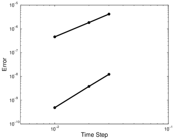
Figure 2: The plot above shows the dependence of the global error, obtained by integrating $P_{1}$ for one full period, on the time step for numerical integrators of $2$nd and $3$rd order. The $2$nd order integrator used was Crank-Nicolson-Adam-Bashforth and the third order method was the $(4,3,3)$ method of (Ascher et al., 1997).

Although the solutions reported in Table 1 are all linearly unstable, they can all be verified using a good DNS code for channel flow as will be shown in this section. We also explain how the error estimates reported in the last column of Table 1 were derived.

The characteristic multipliers $\lambda_{max}$ reported in Table 1 are all greater than $1$ but less than $100$ in magnitude. For characteristic multipliers in that range, the errors due to time discretization can be made negligible. To see that, consider the initial value problem $\dot{x}=f(x)$, $x(0)=x_{0}$. The global error after time $T$ is defined as $\lVert\tilde{x}(T;x_{0})-x(T;x_{0})\rVert$, where $\tilde{x}(T;x_{0})$ is the numerical approximation to the solution $x(T;x_{0})$ at time $T$. For an integrator of order $r$ the global error is asymptotically equal to $E(T)h^{r}$ in the limit of small $h$. Indeed, explicit formulas can be obtained for the function $E(T)$ (Viswanath, 2001). Those formulas indicate that $E(T)$ will increase with $\lambda_{max}$ for the solutions listed in Table 1. However, as indicated by the asymptotic formula and as demonstrated in Figure 2, the global error can be made quite small by taking a small time step. For all the six solutions in Table 1, we carried out computations similar to the one shown in Figure 2 and chose a time step small enough to make the time discretization errors irrelevant. The final computations were all carried out using a $3$rd order implicit-explicit Runge-Kutta method developed by Ascher et al. (1997).

The argument in the previous paragraph would have been invalid if some characteristic multipliers were too large in magnitude. For instance, if $\lambda_{max}>10^{15}$, even the rounding errors would be amplified to an $O(1)$ magnitude over a single cycle. In such situations, one has to use multiple shooting.

Thus if the system $\dot{X}=f(X)$ is obtained by spatially discretizing the Navier-Stokes equation (2.1) and we compute a relative periodic solution of that system with a small enough time step, how close the computed solution is to a true periodic solution of the Navier-Stokes equation is entirely determined by the spatial discretization error.

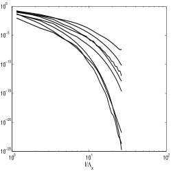
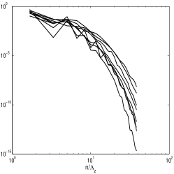
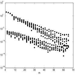
Figure 3: The first two plots show the variation of the energy with streamwise and spanwise wavenumbers, respectively, for the relative periodic solution $P_{6}$. The energies are computed using the slice $y=0$ and at eight equally spaced instants along $P_{6}$’s period. The third plot shows the magnitude of the energy in wall-normal Chebyshev mode against the Chebyshev mode at eight equally spaced instants along $P_{6}$’s period.

We estimate the spatial discretization error in two ways. The first way is to graph energy against streamwise wavenumber, spanwise wavenumber, and wall-normal Chebyshev mode as shown in Figure 3. The first two plots in that figure do not show the energy that corresponds to the wavenumber $0$. Because the Chebyshev polynomials are not orthogonal with respect to the Lebesgue measure, the decomposition of the energy into Chebyshev modes is necessarily somewhat arbitrary. We defined

$$E(y)=\int_{0}^{2\pi\Lambda_{z}}\int_{0}^{2\pi\Lambda_{x}}u(x,y,z)^{2}+v(x,y,z)^{2}+w(x,y,z)^{2}\>dx\,dy,$$

and expressed $E(y)$ as a linear combination of Chebyshev polynomials to get the third plot in Figure 3. More specifically, if $E(y)=\sum_{m=0}^{M}c_{m}T_{m}(y)$, where $T_{m}(y)$ are Chebyshev polnomials, the third plot in Figure 3 plots $\left|c_{m}\right|$ against $m$. Estimates for the discretization error are obtained by taking the square root of the fraction of the energy in the highest mode. Thus we will have streamwise, spanwise, and wall-normal estimates at each point along the relative periodic solution. The worst of these estimates corresponds to the direction that is less well-resolved than the other two, and the instant along the solution where the velocity field is hardest to resolve.

Another possibly more reliable way to estimate the spatial discretization error is to take the initial state of the computed relative periodic solution and then move it to a much finer grid. The initial data is integrated on this finer grid using a sufficiently small time step for one full period. The final state is then shifted using the shifts $s_{x}$ and $s_{z}$. The quantity

$$\frac{\lVert\text{shifted final state}-\text{initial state}\rVert}{\lVert\text{initial state}\rVert}$$

is taken as an estimate of the spatial discretization error.

In all six cases reported in Table 1, these two methods gave comparable estimates for the spatial discretization error. All the errors reported in Table 1 were obtained using the second method and a finer grid with $(2L,M,2N)=(64,90,64)$. As our discussion of time discretization error makes it clear, all the error estimates can be verified using a good DNS code with a sufficiently small time step. Gibson used data about $P_{1}$ that had a relative error of $10^{-5}$ and verified that error estimate using his Channelflow code (Gibson, 2002).

4 Relative periodic solutions and the bursting phenomenon

The most striking thing about the bursting phenomenon in experiments is its recurrent nature. As Acarlar and Smith (1987) state “The study of boundary-layer turbulence in the last thirty years has clearly demonstrated that the chaotic behavior referred to as turbulence has a systematic organization. Most researchers share a common belief that a cyclic bursting phenomenon is the predominant mode of turbulence production.” In this section, we demonstrate the relevance of the periodic and relative periodic solutions listed in Table 1 to the bursting phenomenon.

4.1 Position of relative periodic solutions in phase space

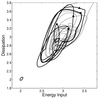
Figure 4: Energy dissipation ($D$) and energy input ($I$) are defined by (2.3) and (2.4). The periodic orbit in the lower left corner is $P_{1}$. The other orbits correspond to the solutions $P_{2}$ through $P_{6}$ with the correspondence given by the markers. The marker for each periodic orbit is listed in Table 1. A random turbulent trajectory is shown in the background.

A good preliminary idea of the relative location of solutions in phase space can be formed by projecting the orbits to the $D$-$I$ plane (Kawahara and Kida, 2001). The normalization used for $D$ and $I$ in (2.3) and (2.4) is such that the laminar solution of plane Couette flow is located at $(1,1)$. We immediately see from Figure 4 that $P_{1}$ is much closer to the laminar solution than the other solutions. As mentioned earlier, $P_{1}$ is not a bursting solution, while the others are.

Greater energy dissipation is connected with steeper gradients in the flow. It is therefore tempting to conclude that orbits that travel farther into the upper-right corner of Figure 4 are harder to resolve. That conclusion is true only approximately. Plots of energy against wavenumber or Chebyshev mode look very similar to Figure 3 for $P_{2}$, $P_{3}$, $P_{4}$, and $P_{5}$, but not for $P_{1}$. The most striking aspect of the plots for $P_{6}$ in Figure 3 lies in the plot of energy against streamwise wavenumber. While at one instant the energy falls by more than a factor of $10^{20}$ over the range of streamwise wavenumbers represented in the computational grid, it falls by only a factor of about $10^{8}$ at another instant. This striking change in energy distribution is directly related to the breakdown of streaks and is observed in $P_{2}$ through $P_{6}$ but not in $P_{1}$.

The existence of periodic and relative periodic solutions is related to two general principles in dynamics, namely the Poincaré recurrence theorem and the closing lemma (Katok and Hasselblatt, 1995). The recurrent nature of the bursting process was observed in direct numerical simulation of plane Couette turbulence and motivated the derivation of the self-sustaining process (Hamilton et al., 1995; Waleffe, 1997). It must be pointed out, however, that the right notion of recurrence in plane Couette flow is not that of periodicity but that of relative periodicity. This is because if an initial velocity field for plane Couette flow is shifted in either the streamwise or the spanwise direction, the final velocity fields after a certain interval of time must be equal to each other after exactly the same shifts. From the point of view of the dynamics, velocity fields that are related by streamwise and spanwise shifts are equivalent.

The same general principles that suggest the existence of periodic and relative periodic solutions that correspond to bursting, also suggest that there will be infinitely many of them. Indeed, these solutions probably give the best or only means to uncover the “systematic organization” found within turbulent boundary layers that Acarlar and Smith refer to in the passage quoted at the beginning of this section. This possibility will be discussed at length in the concluding discussion section.

4.2 Near-wall statistics

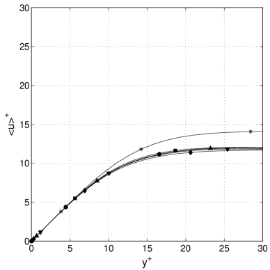
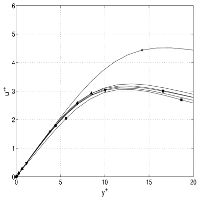
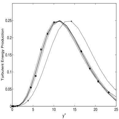
Figure 5: The first of the top two plots shows the dependence of the mean streamwise velocity $<\!\!u\!\!>^{+}$ in wall units upon the distance $y^{+}$ from the upper wall, also in wall units. The second plot shows the dependence of the turbulent intensity as given by the root mean square streamwise velocity $u^{\prime+}$ upon the distance from the wall. The bottom plot shows the dependence of turbulent energy production upon the distance from the wall. The correspondence to the solutions $P_{1}$ through $P_{6}$ listed in Table 1 is shown using markers.

Turbulent boundary layers can be divided into a viscous sublayer, a buffer layer, and a logarithmic boundary layer (Monin and Yaglom, 1971). In the viscous sublayer, which is approximately $5$ wall units thick, the mean streamwise velocity nearly equals the distance from the wall in wall units. The buffer layer extends from $5$ wall units to approximately $25$ or $30$ wall units, and the logarithmic boundary layer begins after that. The viscous stresses dominate in the viscous sublayer, while the Reynolds stresses dominate in the logarithmic boundary layer. Both stresses are significant in the buffer layer.

The first plot in Figure 5 shows the dependence of the mean streamwise velocity upon the distance from the wall. The averages are computed over one single period for each periodic solution in all plots in Figure 5. The law of the wall is reproduced correctly in the viscous sublayer, but the logarithmic boundary layer is not fully developed. The distance between the two moving walls in plane Couette flow in only about $70$ wall units or so for the solutions listed in Table 1, which is one reason the logarithmic boundary layer is not fully developed. Another related reason is that the frictional Reynolds numbers listed in Table 1 are too low for the logarithmic boundary layer to be fully formed. A dynamical investigation of the interaction of structures away from the buffer region with structures in the buffer region can be found in (Itano and Toh, 2005).

The most important features of bursting are in the buffer layer and these features are reproduced correctly by $P_{2}$ through $P_{6}$ as shown by the other two plots in Figure 5. The top-right plot graphs the turbulent intensity against the distance from the wall. The graphs for $P_{2}$ through $P_{6}$ all have the right shape and the turbulent intensity peaks between $10$ and $20$ wall units for each of those solutions. However, the peak is slightly elevated as compared with the theory and experiments recorded in Figure 27 of Monin and Yaglom (1971) or with the “corrected” experiment and computation recorded in Figure 7 of (Kim et al., 1987). This elevation of the peak is a low Reynolds number effect. The peak of the turbulence intensity compares well with Figure 3 of (Jiménez et al., 2005).

The energy balance equation, which is obtained by applying the method of averaging to the Navier-Stokes equation, is important both in theory and in practice (Monin and Yaglom, 1971). Physical interpretations can be associated with the terms of that equation, and we will look at the so-called turbulent energy production term. This term equals

$$-<\!\!u^{\ast}v^{\ast}\!\!>\frac{\partial<\!\!u\!\!>}{\partial y},$$

where $u^{\ast}=u-<\!\!u\!\!>$ and $v^{\ast}=v-<\!\!v\!\!>$ are the fluctuating components of the streamwise and wall-normal velocities and $<\!\!u\!\!>$ is the mean streamwise velocity. In Figure 5, the turbulent energy production is expressed in wall units, although experimentalists do not always use wall units for expressing turbulent energy production (Kline et al., 1967).

Turbulent energy production has a sharp peak in the buffer region for each of $P_{2}$ through $P_{6}$, as shown by the bottom plot in Figure 5. Turbulent energy production can be readily measured in experiments and its sharp peak in the buffer region has intrigued experimentalists for a long time (Kline et al., 1967). The significance of the bursting phenomenon is in part because of its connection to turbulent energy production. We observe from the bottom plot of Figure 5 that for $P_{1}$, which is not a bursting solution, turbulent energy production attains its maximum value farther away from the wall.

4.3 Break-up and advection of coherent structures

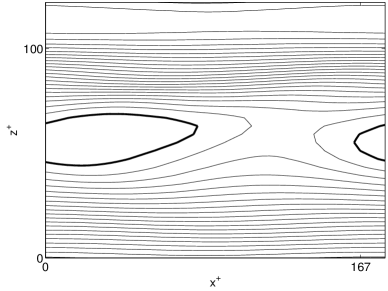
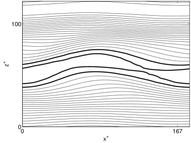
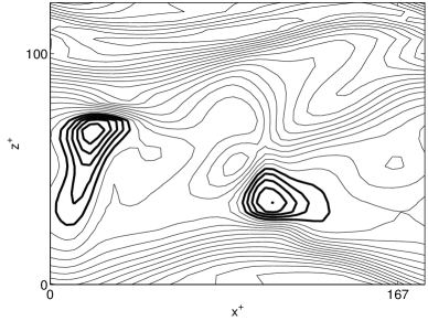
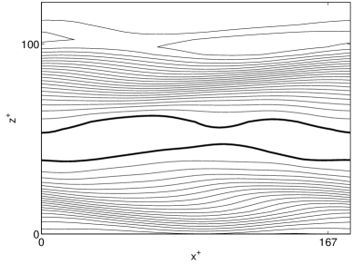
Figure 6: Isolines of the streamwise velocity in the $z$ vs. ​​$x$ plane at $y^{+}\approx 10$ for the relative periodic solution $P_{4}$. The four plots correspond to $t=0,T/4,T/2,3T/4$, where $T$ is the period of $P_{4}$. The plots are in clockwise order, beginning at the top left. The velocity fields were shifted in such a way that a plot at $t=T$ would coincide exactly with the plot for $t=0$. The isolines are thin if the streamwise velocity is positive, and thick if it is negative. Each of the four plots has $24$ isolines equispaced between minimum values which are $-0.5,-1.4,-2.3,-0.5$ (in wall units) and maximum values which are $9.4,9.4,7.5,8.3$.

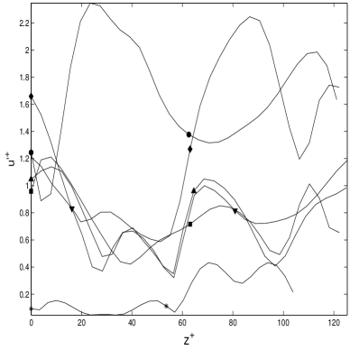
Figure 7: The plot above shows the variation of the root mean square value of the fluctuating part of streamwise velocity, which is denote by $u^{\prime+}$, in the spanwise direction. The rms value is computed at $y^{+}\approx 10$ and $x=\pi\Lambda_{x}$.

Streaks are the most prominent coherent structures observed in turbulent boundary layers. In streaky velocity fields, the streamwise velocity is only weakly dependent on the streamwise coordinate but varies much more strongly in the spanwise direction. In contour plots such as those in Figure 6, streakiness shows up as isolines that are nearly parallel to the $x$ axis. It is clear from that figure that streaks at $t=T/2$ break-up at $t=3T/4$ and then re-form. The plot at $t=0$ corresponds to the initial velocity field of $P_{4}$.

It is difficult to measure the velocity field as a whole in experiments, and therefore experimental visualizations of streaks rely on hydrogen bubbles introduced into the flow by platinum wires and other techniques (Kline et al., 1967; Smith and Metzler, 1983). Sometimes streaks are detected using pointwise measurements (Klebanoff et al., 1962). Figure 7 shows the dependence of the fluctuations of the streamwise velocity on the spanwise direction. The rms velocity $u^{\prime+}$ shown in the top-right plot of Figure 5 was obtained by averaging over a period and by averaging spatially in the spanwise and streamwise directions. But in Figure 7, only the time average was used for computing the rms velocity.

The possibility that the break-up of streaks observed experimentally could be an artifact of flow visualization techniques has been considered by Jiménez et al. (2005). It has been suggested that the advection of permanent objects could be partly responsible for experimental observations. Our computation of relative periodic solutions ($P_{2}$ through $P_{5}$) shows that temporal periodicity and the advection of permanent objects are not mutually exclusive possibilities. While it is generally implicitly assumed that the advection of coherent structures could only be in the streamwise direction, our computation of $P_{2}$ and $P_{4}$ shows that the advection could be in the spanwise direction as well. This could be significant, as will be seen shortly.

The spanwise variation in the strength of the fluctuations of the streamwise velocity shown in Figure 7 for $P_{1}$ through $P_{6}$ is reminiscent of experimental data, such as Figure 2 of (Klebanoff et al., 1962) for instance. This spanwise variation is not very pronounced for $P_{1}$, which is not a bursting solution, but is very pronounced for $P_{2}$ and $P_{4}$. Those are the only two solutions in Table 1 which have a spanwise drift. We are led to conclude that spanwise advection of coherent structures could be a significant source of the observed spanwise variation of $u^{\prime+}$.

4.4 Discrete symmetries of plane Couette flow

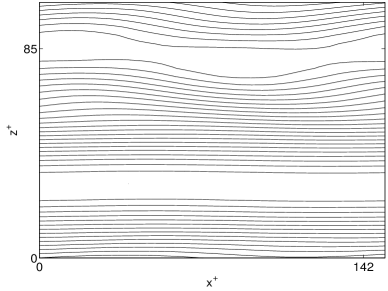
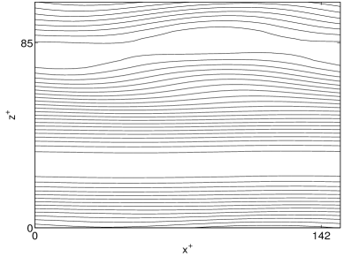
Figure 8: The two plots above show slices through the streamwise velocity field of $P_{1}$ at $t=0$ and $t=T/2$, respectively. The slices were taken at $y^{+}\approx 9$. As explained in the text, the plots show that $P_{1}$ does not have the shift-reflection symmetry. Isolines of $u^{+}$ are drawn at $24$ equispaced values between a maximum of $11.6$ and a minimum of $1.6$. The maximum occurs in the wide gap between isolines in the lower part of either plot, and the minimum occurs in the gap in the upper part.

The Navier-Stokes equation for plane Couette flow has two discrete symmetries (Waleffe, 2003). The shift-reflection transformation of the velocity field is given by

$$\begin{pmatrix}u\\ v\\ w\end{pmatrix}\Biggl{(}x+\pi\Lambda_{x},y,-z\Biggr{)},$$

and the shift-rotation transformation of the velocity field is given by

$$\begin{pmatrix}-u\\ -v\\ w\end{pmatrix}\Biggl{(}-x+\pi\Lambda_{x},-y,z+\pi\Lambda_{z}\Biggr{)}.$$

Plane Couette flow is unchanged under both these transformations. Thus if a single velocity field along a trajectory of plane Couette flow satisfies either symmetry, all points along the trajectory must have the same symmetries. However, velocity fields that lie on the stable and unstable manifolds of symmetric periodic or relative periodic solutions need not be symmetric.

Figure 8 shows that $P_{1}$ does not have the shift-reflection symmetry. Both the plots would look very different if they were flipped upside-down and shifted forward by half the width of the plot in the $x$ direction. We have verified that $P_{1}$ does not have the shift-rotation symmetry either. A close inspection of Figure 8 reveals that the second plot can be obtained by shifting the first plot in the $x$ direction. In fact, $P_{1}$ is a relative periodic solution. During half the period listed in Table 1, the initial velocity field of $P_{1}$ shifts by $s_{x}/\pi\Lambda_{x}=0.5$ and $s_{z}=0$.

The averaged velocity field of a long turbulent trajectory of plane Couette flow satisfies the discrete symmetries to a very rough approximation. However, there is no reason to believe that such an average has any dynamical significance. The average could just be a transient state and it may not even lie on the asymptotic set of the flow.

The six solutions listed in Table 1 satisfy neither the shift-reflection symmetry nor the shift-rotation symmetry. This implies that the shift-reflection and shift-rotation transformations (which commute with each other) can be applied to each solution in Table 1 to obtain $18$ more solutions.

4.5 Unstable manifolds of the solutions $P_{i}$

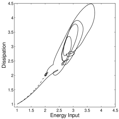
Figure 9: The plot above shows the projection of the unstable manifold of $P_{1}$ to the energy dissipation vs.​​ energy input plane.

In their study of the bursting phenomenon in turbulent Poiseuille flow, Itano and Toh (2001) found that the break-up and re-formation of coherent structures is well approximated by the unstable manifold of a traveling wave solution. Among the solutions we have computed, $P_{1}$ most resembles the traveling wave solution of (Itano and Toh, 2001). Motivated by that resemblence, we asked if the solutions $P_{2}$ through $P_{6}$ could be related to the unstable manifold of $P_{1}$.

We perturbed $P_{1}$ along the single unstable direction that corresponds to that solution. A perturbation in one sense begins to head towards the laminar solution right away and falls into the laminar solution. A perturbation with the opposite sign heads into the turbulent region, as shown in Figure 9 but relaminarizes eventually. In contrast, we found that perturbations along the unstable manifolds of the bursting periodic solutions $P_{2}$ through $P_{6}$ do not relaminarize. Thus there appears to be no relationship between the unstable manifold of $P_{1}$ and the other solutions.

In addition, unlike $P_{1}$ the bursting solutions have more than one unstable direction. For instance, the Arnoldi iteration shows that $P_{2}$ has at least $11$ unstable directions. These facts suggest that the unstable manifold of $P_{1}$ cannot by itself explain the bursting phenomenon in the plane Couette scenario considered in this paper.

5 Discussion

The approach to the bursting phenomenon, and to turbulence in fluid flows more generally, that this paper advocates is quite simple. As the incompressible Navier-Stokes equation is an excellent physical model, our approach is simply to compute solutions of that differential equation. This approach should not be surprising in itself because the main reason for deriving differential equations is to understand their solutions. However, well-resolved spatial discretizations of turbulent phenomena require more than a hundred thousand degrees of freedom and computing solutions with so many degrees of freedom is nontrivial. We have shown that problems associated with largeness of the number of degrees of freedom can be overcome. Indeed, our computations of periodic and relative periodic solutions used as many as twenty times the number of degrees of freedom in any earlier computation of periodic solutions.

Having decided to compute solutions, one must decide what type of solutions to look for within turbulent flows. Here the basic principles of dynamics are of help. The recurrent nature of the bursting phenomenon has been noted by experimentalists, as we pointed out earlier. Recurrence, which is the tendency of certain dynamical systems to revisit points close to their initial state in phase space after extended excursions, has long been a central and unifying idea in dynamics. The relevance of recurrence to long term dynamics is captured in a most general way by the Poincaré recurrence theorem (Katok and Hasselblatt, 1995). In its early days, this theorem gave rise to troubling questions about the foundations of statistical mechanics. The number of degrees of freedom needed for resolving low Reynolds number turbulence is quite large, yet far smaller than the number of degrees of freedom typical of statistical mechanics. Another significant difference is that low Reynolds number turbulence is governed by equations that are not Hamiltonian and in which viscosity damps high wavenumbers. Therefore there is reason to think that a point of view based on recurrences will be useful for understanding turbulence.

A combination of local instability, which is a well-known feature of turbulent flows, and boundedness in phase space naturally suggests the existence of periodic motions. The closing lemma is a principle that suggests that dynamics can be understood quite generally in terms of periodic solutions (Katok and Hasselblatt, 1995). It has been proved in a few restricted settings and serves as a beacon. While considering the closing lemma, it is worth noting again that the right notion of recurrence depends upon invariance properties of the underlying differential equation. If the differential equation is unchanged by a continuous group of transformations, then it is appropriate to look for relative periodic solutions.

In some well-understood settings, it is possible to prove the existence of infinitely many periodic solutions (Moser, 1973). Even though turbulent phenomena are not known to fall under any of these settings, there is reason to think that there are infinitely many periodic and relative periodic solutions embedded within turbulent flows. The lack of complete theoretical results should not be an impediment to computation, since the major purpose of computation is to render tractable problems that are beyond the reach of theory. An advantage of computing many of these solutions is that they can help us understand the dynamics as a whole in terms of accurately computed periodic solutions. In addition, these periodic solutions could serve as a basis to understand turbulent statistics using the periodic orbit theory (Cvitanović et al., 2005).

It is natural to expect different solutions of the same differential equation to bear a relationship to one another. In the case of linear differential equations, the principle of linear superposition gives this relationship. For chaotic nonlinear systems, the relationship between solutions is much more complicated and intriguing. In several instances, the precise nature of the relationship is given by symbolic dynamics (Moser, 1973). Algorithms for computing nonlinear systems can be based upon symbolic dynamics (Viswanath, 2003, 2004). Those algorithms made it possible to compute the fractal structure of the well-known Lorenz attractor. Although the fractal structure of the Lorenz attractor was deduced by Lorenz (1963), its computation became possible only with algorithms based on symbolic dynamics. The Lorenz equations were derived to illuminate the essentially deterministic nature of turbulence and they have been completely successful in that respect. Computations of the strange attractor of the Lorenz equations can likewise serve as models for computations of turbulence.

The Lorenz computations based on symbolic dynamics illustrate the advantanges of periodic solutions over steady solutions in understanding the dynamics as a whole. It is possible to accurately compute periodic solutions that are as close as machine precision permits to random points on the Lorenz attractor, and thus obtain a very good understanding of the dynamics (Viswanath, 2003). Such a precise understanding cannot be obtained using steady solutions alone. To understand important aspects of turbulent boundary layers such as the turbulent energy production in the buffer layer, it is likewise necessary to go beyond steady solutions and traveling waves and compute periodic and relative periodic solutions.

It would be premature to suggest that the various solutions embedded within turbulent flows can be described using symbolic dynamics. Yet, it would be very surprising if these solutions did not bear a relationship to one another. Discovering such a relationship would be a major advance in our understanding of turbulent flows.

This paper has asserted the existence of six solutions of turbulent plane Couette flow. Error estimates for these solutions were supplied in Table 1. We argued in Section 3 that these solutions, along with their error estimates, can be verified using a good code for direct numerical simulation of channel flows. Such quantitative reproducibility is a step forward in the area of turbulence computation.

6 Acknowledgments

The author thanks P. Cvitanović and F. Waleffe for many helpful discussions; J.F. Gibson for checking some of the solutions using his Channelflow code; and G. Kawahara and S. Toh for clarifications. This work was supported by the NSF grant DMS-0407110 and by a research fellowship from the Sloan Foundation.

Data for solutions reported in this article can be obtained by contacting the author.

References

- Acarlar and Smith (1987) M.S. Acarlar and C.R. Smith. A study of hairpin vortices in a laminar boundary layer. Journal of Fluid Mechanics, 175:1–83, 1987.
- Ascher et al. (1997) U.M. Ascher, S.J. Ruuth, and R.J. Spiteri. Implicit-explicit Runge-Kutta methods for time-dependent partial differential equations. Applied Numerical Mathematics, 25:151–167, 1997.
- Bech et al. (1995) K.H. Bech, N. Tillmark, P.H. Alfredsson, and H.I. Andersson. An investigation of turbulent plane Couette flow at low Reynolds number. Journal of Fluid Mechanics, 286:291–325, 1995.
- Cvitanović et al. (2005) P. Cvitanović, R. Artuso, R. Mainieri, G. Tanner, and G. Vattay. Chaos: Classical and Quantum. ChaosBook.org, Niels Bohr Institute, Copenhagen, 2005.
- Dennis and Schnabel (1996) J.E. Dennis and R.B. Schnabel. Numerical Methods for Unconstrained Optimization and Nonlinear Equations. SIAM, Philadelphia, 1996.
- Faisst and Eckhardt (2003) H. Faisst and B. Eckhardt. Traveling waves in pipe flow. Physical Review Letters, 91:art. 224502, 2003.
- Gibson (2002) J.F. Gibson. Dynamical systems models of wall-bounded, shear-flow turbulence. PhD thesis, Cornell University, 2002.
- Hamilton et al. (1995) J.M. Hamilton, J. Kim, and F. Waleffe. Regeneration mechanisms of near-wall turbulence structures. Journal of Fluid Mechanics, 287:317–348, 1995.
- Hof et al. (2004) B. Hof, C.W.H. van Doorne, et al. Experimental observation of nonlinear traveling waves in turbulent pipe flows. Science, 305:1594–1598, 2004.
- Holmes et al. (1996) P. Holmes, J.L. Lumley, and G. Berkooz. Turbulence, Coherent Structures, Dynamical Systems, and Symmetry. Cambridge Univeristy Press, Cambridge, 1996.
- Itano and Toh (2001) T. Itano and S. Toh. The dynamics of bursting process in wall turbulence. Journal of the Physical Society of Japan, 70:701–714, 2001.
- Itano and Toh (2005) T. Itano and S. Toh. Interaction between large-scale structure and near-wall structures in channel flow. Journal of Fluid Mechanics, 524:249–262, 2005.
- Jiménez et al. (2005) J. Jiménez, G. Kawahara, M.P. Simens, M. Nagata, and M. Shiba. Characterization of near-wall turbulence in terms of equilibrium and bursting solutions. Physics of Fluids, 17:art. 015105, 2005.
- Katok and Hasselblatt (1995) A. Katok and B. Hasselblatt. Introduction to the Modern Theory of Dynamical Systems. Cambridge University Press, Cambridge, 1995.
- Kawahara (2005) G. Kawahara. Laminarization of minimal plane Couette flow: going beyond the basin of attraction of turbulence. Physics of Fluids, 17:art. 041702, 2005.
- Kawahara and Kida (2001) G. Kawahara and S. Kida. Periodic motion embedded in plane Couette turbulence: regeneration cycle and burst. Journal of Fluid Mechanics, 449:291–300, 2001.
- Kelley (2003) C.T. Kelley. Solving Nonlinear Equations with Newton’s Method. SIAM, Philadelphia, 2003.
- Kerswell (2005) R.R. Kerswell. Recent progress in understanding the transition to turbulence in a pipe. Nonlinearity, 18:R17–R44, 2005.
- Kim et al. (1987) J. Kim, P. Moin, and R. Moser. Turbulence statistics in fully developed channel flow at low Reynolds number. Journal of Fluid Mechanics, 177:133–166, 1987.
- Klebanoff et al. (1962) P.S. Klebanoff, K.D. Tidstrom, and L.M. Sargent. The three dimensional nature of boundary layer instability. Journal of Fluid Mechanics, 12:1–34, 1962.
- Kline et al. (1967) S.J. Kline, W.C. Reynolds, F.A. Schraub, and P.W. Rundstadler. The structure of turbulent boundary layers. Journal of Fluid Mechanics, 30:741–773, 1967.
- Lorenz (1963) E.N. Lorenz. Deterministic non-periodic flow. J. Atmos. Sci., 20:130–141, 1963.
- Monin and Yaglom (1971) A.S. Monin and A.M. Yaglom. Statistical Fluid Mechanics. The MIT Press, Cambridge, 1971.
- Moser (1973) J. Moser. Stable and Random Motions in Dynamical Systems. Princeton University Press, New Jersey, 1973.
- Sancheź et al. (2004) J. Sancheź, M. Net, B. Garćia-Archilla, and C. Simó. Newton-Krylov continuation of periodic orbits for Navier-Stokes flows. Journal of Computational Physics, 201:13–33, 2004.
- Schoppa and Hussain (2002) W. Schoppa and F. Hussain. Coherent structure generation in near-wall turbulence. Journal of Fluid Mechanics, 453:57–108, 2002.
- Smith and Metzler (1983) C.R. Smith and S.P. Metzler. The study of hairpin vortices in a laminar boundary layer. Journal of Fluid Mechanics, 129:27–54, 1983.
- Trefethen and Bau (1997) L.N. Trefethen and D. Bau. Numerical Linear Algebra. SIAM, Philadelphia, 1997.
- Viswanath (2001) D. Viswanath. Global errors of numerical ODE solvers and Lyapunov’s theory of stability. IMA Journal of Numerical Analysis, 21:387–406, 2001.
- Viswanath (2003) D. Viswanath. Symbolic dynamics and periodic orbits of the Lorenz attractor. Nonlinearity, 16:1035–1056, 2003.
- Viswanath (2004) D. Viswanath. The fractal property of the Lorenz attractor. Physica D, 190:115–128, 2004.
- Waleffe (1997) F. Waleffe. On a self-sustaining process in shear flows. Physics of Fluids, 9:883–900, 1997.
- Waleffe (1998) F. Waleffe. Three-dimensional coherent states in plane shear flows. Physical Review Letters, 81:4140–4143, 1998.
- Waleffe (2001) F. Waleffe. Exact coherent structures in channel flow. Journal of Fluid Mechanics, 435:93–102, 2001.
- Waleffe (2003) F. Waleffe. Homotopy of exact coherent structures in plane shear flows. Physics of Fluids, 15:1517–1534, 2003.
- Wedin and Kerswell (2004) H. Wedin and R.R. Kerswell. Exact coherent structures in pipe flow: travelling wave solutions. Journal of Fluid Mechanics, 508:333–371, 2004.