Phenomenological Models of Socio-Economic Network Dynamics

Abstract

We study a general set of models of social network evolution and dynamics. The models consist of both a dynamics on the network and evolution of the network. Links are formed preferentially between ’similar’ nodes, where the similarity is defined by the particular process taking place on the network. The interplay between the two processes produces phase transitions and hysteresis, as seen using numerical simulations for three specific processes. We obtain analytic results using mean field approximations, and for a particular case we derive an exact solution for the network. In common with real-world social networks, we find coexistence of high and low connectivity phases and history dependence.

I Introduction

In recent years physicists have paid much attention to network structures – describing either technological infrastructures or biological, genetic, logical or social relationships – as they play a prominent role in shaping the nature of the processes taking place on them and the resulting collective behavior. Examples of how the structure affects the function of networked systems include the importance of shortcuts in endowing finite dimensional networks of the small world property WattsStrogatz and of scale-free degree distribution for robustness against failure Cohen or the relevance of motifs for specific dynamical properties motifs .

Socio-economic networks offer an example where the relation between structure and function is not unidirectional. Indeed their structure is inherently dynamical and it is shaped by the incentives of agents, i.e. by the socio-economic functions provided by the network. This paper discusses a class of generic model of stochastic dynamical social networks which make the interplay between structure and function of social network explicit in a simple way. We consider a set of agents – be they individuals or organisations – who establish bilateral interactions (links) when profitable. The network evolves under changing conditions. That is, the favourable circumstances that led at some point to the formation of a particular link may later on deteriorate, causing that link’s removal. Hence volatility (exogenous or endogenous) is a key disruptive element in the dynamics. Concurrently, new opportunities arise that favour the formation of new links. Whether linking occurs depends on factors related to the similarity or proximity of the two parties. For example, in cases where trust is essential in the establishment of new relationships (e.g. in crime or trade networks), linking may be facilitated by common acquaintances or by the existence of a chain of acquaintances joining the two parties. In other cases (e.g. in R&D or scientific networks), a common language, methodology, or comparable level of technical competence may be required for the link to be feasible or fruitful to both parties.

In a nutshell, our model conceives the dynamics of the network as a struggle between volatility (that causes link decay) on the one hand, and the creation of new links (that is dependent on similarity) on the other. The model must also specify the dynamics governing inter-node similarity. A reasonable assumption in this respect is that such similarity is enhanced by close interaction, as reflected by the social network. For example, a firm (or researcher) benefits from collaborating with a similarly advanced partner, or individuals who interact regularly tend to converge on their social norms and other standards of behavior.

We study different specifications of the general framework, each one embodying alternative forms of the intuitive idea that “interaction promotes similarity.” Our main finding is that in all of these different cases the network dynamics exhibits a rich phenomenology characterized by a) sharp phase transition b) resilience, i.e. stability against deteriorating conditions and c) equilibrium coexistence. The essential mechanism at work is a positive feedback between link creation and inter-node similarity, these two factors each exerting a positive effect on the other. Feedback forces of this kind appear to operate in the dynamics of many social networks. We show that they are sufficient to produce the sharp transitions, resilience, and equilibrium co-existence that, as we will discuss in the next section, are salient features of many socio-economic phenomena. Finally, this phenomenology bears a formal similarity with the liquid-gas phase transition, thus suggesting that a classification in terms of phases may be applicable also to socio-economic networks.

The rest of this paper is organized as follows: The next section discusses in an introductory way the empirical evidence which our model addresses. In section III we outline the general setup and a generic model of which we will discuss particular realizations the following sections. In particular, we shall first discuss the case where network formation depends on the topology of the network (sect. IV) and then cases where it is coupled with the dynamics of a continuous (sect. V) or discrete (sect. VI) variable. These two models addresses situations where homogeneity in some dimension (e.g. technological levels or knowledge) or coordination (on e.g. a standard) play a crucial role, respectively. Numerical simulations will be supplemented by mean field analysis which provides a correct qualitative picture in all cases and, in some cases, accurate quantitative estimates. A case where an exact solution can be derived will be described in section VII. In section VIII we end with some concluding remarks.

II Empirical stylized facts of socio-economic networks

There is a growing consensus among social scientists that many social phenomena display an inherent network dimension. Not only are they “embedded” in the underlying social network Granov but, reciprocally, the social network itself is largely shaped by the evolution of those phenomena. The range of social problems subject to these considerations is wide and important. It includes, for example, the spread of crime Glaeseretal ; Haynie and other social problems (e.g. teenage pregnancy Crane ; Harding ), the rise of industrial districts OECD ; Saxenian ; Granovetteretal , and the establishment of research collaborations, both scientific Newman ; Goyaletal and industrial Hagedoorn ; Kogut . Throughout these cases, there are a number of interesting observations worth highlighting:

(a) Sharp transitions: The shift from a sparse to a highly connected network often unfolds rather “abruptly,” i.e. in a short timespan. For example, concerning the escalation of social pathologies in some neighborhoods of large cities, Crane Crane writes that “…if the incidence [of the problem] reaches a critical point, the process of spread will explode.” Also, considering the growth of research collaboration networks, Goyal et al. Goyaletal report a steep increase in the per capita number of collaborations among academic economists in the last three decades, while Hagerdoorn Hagedoorn reports an even sharper (ten-fold) increase for R&D partnerships among firms during the decade 1975-1985.

(b) Resilience: Once the transition to a highly connected network has taken place, the network is robust, surviving even a reversion to “unfavorable” conditions. The case of California’s Silicon Valley, discussed in a classic account by Saxenian Saxenian , illustrates this point well. Its thriving performance, even in the face of the general crisis undergone by the computer industry in the 80’s, has been largely attributed to the dense and flexible networks of collaboration across individual actors that characterized it. Another intrinsically network-based example is the rapid recent development of Open-Source software (e.g. Linux), a phenomenon sustained against large odds by a dense web of collaboration and trust Benkler . Finally, as an example where “robustness” has negative rather than positive implications, Crane Crane describes the difficulty, even with vigorous social measures, of improving a local neighborhood once crime and other social pathologies have taken hold.

(c) Equilibrium co-existence: Under apparently similar environmental conditions, social networks may be found both in a dense or sparse state. Again, a good illustration is provided by the dual experience of poor neighborhoods in large cities Crane , where neither poverty nor other socio-economic conditions (e.g. ethnic composition) can alone explain whether or not there is degradation into a ghetto with rampant social problems. Returning to R&D partnerships, empirical evidence Hagedoorn shows a very polarized situation, almost all R&D partnerships taking place in a few (high-technology) industries. Even within those industries, partnerships are almost exclusively between a small subset of firms in (highly advanced) countries footnote1 .

From a theoretical viewpoint, the above discussion raises the question of whether there is some common mechanism at work in the dynamics of social networks that, in a wide variety of different scenarios, produces the three features explained above: (a) discontinuous phase transitions, (b) resilience, and (c) equilibrium coexistence. Our aim in this paper is to shed light on this question within a general framework that is flexible enough to accommodate, under alternative concrete specifications, a rich range of social-network dynamics.

III The model

Consider a set ${\cal N}=\{1,\ldots,n\}$ of agents, whose state and interactions evolve in continuous time $t$. They form the nodes of a network which is described by a non-directed graph $g(t)\subset\{ij:i\in{\cal N},~{}j\in{\cal N}\}$, where $ij(\equiv ji)\in g(t)$ iff a link exists between agents $i$ and $j$. The network evolution is modelled in terms of continuous time stochastic elementary Poisson processes, and it is therefore defined by specifying the rates at which these processes occur footnote2 . Firstly, each node $i$ receives an opportunity to form a link with a node $j$, randomly drawn from ${\cal N}$ ($i\neq j$), at rate $\eta$. If the link $ij$ is not already in place, it forms with probability

$$P\{ij\rightarrow g(t)\}=\left\{\begin{array}[]{cc}1&\;\textrm{if }d_{ij}(t)\leq\bar{d}\\ \epsilon&\;\textrm{if }d_{ij}(t)>\bar{d}\end{array}\right.$$ (1)

where $d_{ij}(t)$ is the “distance” (to be specified later) between $i$ and $j$ prevailing at $t.$ Thus if $i$ and $j$ are close, in the sense that their distance is no higher than some given threshold $\bar{d}$, the link forms at rate $\eta$; otherwise, it forms at a much smaller rate $\eta\epsilon$. Secondly, each existing link $ij\in g(t)$ decays at rate $\lambda$. That is, each link in the network disappears with probability $\lambda dt$ in a time interval $[t,t+dt)$. We shall discuss three different specifications of the distance $d_{ij}$, each capturing different aspects that may be relevant for socio-economic interactions.

In all three cases, we mostly focus on the stationary state behavior, which we shall illustrate using both numerical simulations and a mean-field analytic approach. Concerning the latter, we focus on the limit $n\rightarrow\infty$, for which the analysis is simpler. We characterise the long run behavior of the network solely in terms of the stationary degree distribution $p(k)$, which is the fraction of agents with $k$ neighbours. This corresponds to neglecting degree correlations, i.e. to approximating the network with a random graph (see randomGraph ), an approximation which is reasonably accurate in the cases we discuss here. The degree distribution satisfies a master equation, which is specified in terms of the transition rates $w(k\rightarrow k\pm 1)$ for the addition or removal of a link, for an agent linked with $k$ neighbours. While $w(k\rightarrow k-1)=\lambda k$ always takes the same form, the transition rate for the addition of a new link

$$w(k\rightarrow k+1)=2\eta\left[\epsilon+(1-\epsilon)P\{d_{i,j}\leq\bar{d}\}\right]$$

depends on the particular specification of the distance $d_{ij}$. Matching the link creation and removal processes, yields an equation for the degree distribution $p(k)$. The probability $P\{d_{i,j}\leq\bar{d}\}$, in its turn, will itself depend on the network density, i.e. on $p(k)$. Our approach will then have the flavor of a self-consistent mean field approximation.

IV Similarity by (chains of) acquaintances

Consider first the simplest possible such specification where $d_{ij}(t)$ is the (geodesic) distance between $i$ and $j$ on the graph $g(t)$, neighbours $j$ of $i$ having $d_{ij}(t)=1$, neighbours of the neighbours of $i$ (which are not neighbours of $i$) having $d_{ij}(t)=2,$ and so on. If no path joins $i$ and $j$ we set $d_{ij}(t)=\infty$.

This specific model describes a situation where the formation of new links is strongly influenced by proximity on the graph. It is a simple manifestation of our general idea that close interaction brings about similarity – here the two metrics coincide. We set $\bar{d}\geq n-1$, the link formation process then discriminates between agents belonging to the same network component (which are joined by at least one path of links in $g$) and agents in different components. Distinct components of the graph may, for example, represent different social groups. Then Eq. (1) captures the fact that belonging to the same social group is important in the creation of new links (say, because it facilitates control or reciprocity Coleman ; An ).

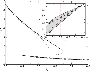
Figure 1: Mean degree $\left<k\right>$ as a function of $\lambda$ ($\eta$ has been set to $1$) for $\epsilon=0.2$ when $d_{ij}$ is the distance on the graph and $\bar{d}\geq n-1$. The results of a mean field theory for $n=\infty$ (solid line) are compared to numerical simulations ($\times$) starting from both low and high connected states with $n=20000$. The dashed line corresponds to an unstable solution of the mean field equations which separates the basins of stability of the two solutions. For finite $n$ the low density state “flips” to the high density state when a random fluctuation in $\left<k\right>$ brings the system across the stability boundary (i.e. when a sizable giant component forms). These fluctuations become more and more rare as $n$ increases. Inset : Phase diagram in mean field theory. Coexistence occurs in the shaded region whereas below (above) only the dense (sparse) network phase is stable. Numerical simulations (symbols) agree qualitatively with the mean field prediction. The high (low) density state is stable up (down) to the points marked with $\times$ ($\diamond$) and is unstable at points marked with $\circ$ ($+$). The behavior of $\left<k\right>$ along the dashed line is reported in the main figure.

Consider first what happens when $\eta/\lambda$ is small. Let $\left<k\right>$ be the average connectivity (number of links per node) in the network. The average rate $n\lambda\left<k\right>/2$ of link removal is very high when $\left<k\right>$ is significant. Consequently, we expect to have a very low $\left<k\right>$, which in turn implies that the population should be fragmented into many small groups. Under these circumstances, the likelihood that an agent $i$ “meets” an agent $j$ in the same component is negligible for large populations, and therefore new links are created at a rate equal to $n\eta\epsilon$. By balancing link creation and link destruction, the average number of neighbours of an agent is $\left<k\right>=2\eta\epsilon/\lambda$, as is indeed found in our simulations (Fig 1).

As $\eta/\lambda$ increases, the network density $\left<k\right>$ increases gradually. Then, at a critical value $(\eta/\lambda)_{1}=1/2\epsilon$ – when $\left<k\right>=1$ – a giant component forms. The system makes a discontinuous jump (Fig. 1) to a state containing a large and densely interconnected community covering a finite fraction of the population. If $\eta/\lambda$ decreases back again beyond the transition point $(\eta/\lambda)_{1}$, the dense network remains stable. The dense network dissolves back into a sparsely connected one only at a second point $(\eta/\lambda)_{2}$. This phenomenology characterises a wide region of parameter space (see inset of Fig. 1) and is qualitatively well reproduced by a simple mean field approach.

It is worth mentioning that a similar phenomenology occurs when $\bar{d}=2$, i.e. when links are preferentially formed with “friends of friends ”matteocomment . In this case, however, the probability that two arbitrary nodes $i$ and $j$ have $d_{ij}=2$ is of order $1/n$ in a network with finite degree. Hence for finite $\epsilon$ and $\lambda$ non-linear effect manifest only for networks of finite sizes matteocomment .

We finally mention that the model with $\bar{d}=2$ is reminiscent of a model that was recently proposed PNAS to describe a situation where (as e.g. in job search Job ) agents find new linking opportunities through current partners. In PNAS agents use their links to search for new connections, whereas here existing links favour new link formation. In spite of this conceptual difference, the model in Ref. PNAS also features the phenomenology (a)-(c) above, i.e. sharp transitions, resilience, and phase coexistence.

IV.1 Mean Field Analysis

The transition rate for the addition of a new link is $w(k\rightarrow k+1)=2\eta\epsilon$ if the two agents are in different components and $w(k\rightarrow k+1)=2\eta$ if they are in the same component, where the factor $2$ comes because each node can either initiate or receive a new link. In the large $n$ limit the latter case only occurs with some probability if the graph has a giant component $\mathcal{G}$ which contains a finite fraction $\gamma$ of nodes. For random graphs (see Ref. randomGraph for details) the fraction of nodes in $\mathcal{G}$ is given by

$$\gamma=1-\phi(u)$$ (2)

where

$$\phi(s)=\sum_{k}p(k)s^{k}$$ (3)

is the generating function and $u$ is the probability that a link, followed in one direction, does not lead to the giant component. The latter satisfies the equation

$$u=\phi^{\prime}(u)/\phi^{\prime}(1).$$ (4)

Hence $u^{k}$ is the probability an agent with $k$ neighbours has no links connecting him to the giant component, and hence is itself not part of the giant component. Then the rate of addition of links takes the form

$$w(k\rightarrow k+1)=2\eta[\epsilon+(1-\epsilon)\gamma(1-u^{k})].$$ (5)

The stationary state condition of the master equation leads to the following equation for $\phi(s)$

$$\lambda\phi^{\prime}(s)=2\eta[\epsilon+(1-\epsilon)\gamma]\phi(s)-2\eta(1-\epsilon)\gamma\phi(us)$$ (6)

which can be solved numerically to the desired accuracy. Notice that Eq. (6) is a self-consistent problem, because the parameters $\gamma$ and $u$ depend on the solution $\phi(s)$. The solution of this equation is summarised in Fig. 1. Either one or three solutions are found, depending on the parameters. In the latter case, the intermediate solution is unstable (dashed line in Fig. 1), and it separates the basins of attraction of the two stable solutions within the present mean field theory.

The solution is exact where there is no giant component, and numerical simulations show that the mean field approach is very accurate away from the phase transition from the connected to the disconnected state. Near the transition to the disconnected state our approximation, that an agent’s degree fully specifies its state, breaks down. This causes the theory to overestimate the size of the coexistence region.

V Similarity of Knowledge/Technology levels

Next, we consider a setup where $d_{ij}$ reflects proximity of nodes $i$, $j$ in terms of some continuous (non-negative) real attributes, $h_{i}(t)$, $h_{j}(t)$. This case has been dealt with in Ref. IJGT , which provides a detailed socio-economic motivation for the model. In short, the attribute $h_{i}$ could represent the level of technical expertise of two firms involved in an R&D partnership, or the competence of two researchers involved in a joint project. It could also be a measure of income or wealth that bears on the quality and prospects of a bilateral relationship. We assume that each agent $i$ receives an attribute update (or upgrade) possibility at a rate $\nu$. We focus on the case where the dynamics of $h_{i}$ is much faster than that of the network ($\nu\gg\lambda,\eta$). In the opposite limit, links exits for too short a time span to have any correlated effect on the dynamics of $h_{i}$. If agent $i$ receives an update opportunity at time $t$, we posit that

$$h_{i}(t^{+})=D\{h_{j},~{}j\in{\cal N}_{i}(t)\}+\eta_{i}(t)$$ (7)

where $\eta_{i}(t)$ is a random term capturing the idiosyncratic change of expertise due to $i$’s own (say research) efforts. In Eq. (7) the function $D\{\cdot\}$ captures some process of diffusion (e.g. sharing of knowledge) in the current neighborhood $\mathcal{N}_{i}(t)=\{j:~{}ij\in g(t)\}$ of agent $i$.

We will take $\eta_{i}(t)$ to be Gaussian i.i.d. random variables with zero mean and variance $\Delta$. This random idiosyncratic term competes with the homogenising force of diffusion described by the first term in Eq. (7). Concerning this term, we will consider two alternative models.

V.1 Best-Practise imitation

The first one, which we will label Best-Practise Imitation (BPI) has the revising player achieve a knowledge level equal to the maximum available in her neighbourhood. We have in mind a situation where individuals aim at improving in the direction of increasing $h_{i}$ and they may do this by some on-site effort and also by learning from other individuals.

Formally, this is captured by the following definition:

$$D\{h_{j},~{}j\in{\cal N}_{i}(t)\cup\{i\}\}=\max_{j\in\mathcal{N}_{i}(t)}h_{j}(t).$$ (8)

Notice that if $i$ has no neighbor ($\mathcal{N}_{i}(t)=\emptyset$) then $D=h_{i}$. This is equivalent to a directed polymer at zero temperature on the (dynamic) network $g(t)$ DPRM . A related model, using the idea of best practice imitation but with different noise has been studied in majumdar , but for randomly chosen neighbours at each interaction (i.e. no network).

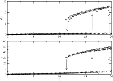
Figure 2: Mean degree $\left<k\right>$ (top) and growth rate $v$ (bottom) as a function of $\eta$, found from numerical simulations of the model with Eq. (8). Shown are simulations with $n=500$ (plusses) and $1000$ (crosses). Arrows denote the approximate point at which the system jumps from one phase to the other (this point can be dependent on $n$). Here $\epsilon=0.001$, noise strength $\Delta=0.1$, similarity threshold $\bar{d}=2$. The system was run up to $t=1000$ for equilibration, then from $t=1000$ to $t=1100$ for data taking.

Fig. 2 reports typical results of simulations of this model. As in the two previous models, we find a discontinuous transition between a sparse and a dense network state, characterised by hysteresis effects. When the network is sparse, diffusion is ineffective in homogenising growth. Hence the distance $d_{ij}$ is typically beyond the threshold $\bar{d}$, thus the link formation process is slow. On the other hand, with a dense network, diffusion keeps the gaps between the $h_{i}$s of different nodes small, which in turn has a positive effect on network formation. As before, the phase transition and hysteresis is a result of the positive feedback that exists between the dynamics of the $h_{i}$ and the adjustment of the network. In the stationary state we find that $h(t)\equiv\left\langle h_{i}(t)\right\rangle$ grows linearly in time, i.e. $h_{i}(t)\simeq vt$. Notably, the growth process is much faster (i.e. $v$ is much higher) in the dense network equilibrium than in the sparse one, as shown in the lower panel of Fig. 2.

This model exhibits an interplay between the process on the network - the $h_{i}(t)$ which depends on the network - and the network evolution which depends on the $h_{i}(t)$. It is this interdependence and the corresponding positive feedback which produces the discontinuous transition and phase coexistence.

The similarity of the behavior of this model with that of the previous section can be understood by analyzing a particular limit. Consider indeed the case where $\eta_{i}=1$ with probability $a$ and $\eta_{i}=0$ otherwise. When $\nu a\ll\eta$ innovations take place at a rate much smaller that that over which new links form. In the limit where the dynamics of $h_{i}$ is fast enough ($\nu\gg\eta$), we can assume that each new innovation (i.e. each event $\eta_{i}=1$) taking place on a connected component instantaneously propagates to the entire set of connected nodes. Hence, if $\bar{d}<1$, link creation will occur with probability one on nodes in the same connected component, whereas nodes in different components will likely have distinct values of $h_{i}$, so that links will form at rate $\eta\epsilon$. Note also that, in this particular limit, the growth rate $v$ is proportional to the size of the largest connected component.

V.2 Conforming to neighbors

The second alternative considered has diffusion embody a uniform merging of the neighbourhood’s levels, formalised as follows

$$D\{h_{j}\}=\left\{\begin{array}[]{cc}\frac{1}{|\mathcal{N}_{i}|}\sum_{j\in\mathcal{N}_{i}(t)}h_{j}(t)&\mathcal{N}_{i}(t)\not=\emptyset\\ h_{i}&\mathcal{N}_{i}(t)=\emptyset\end{array}\right.$$ (9)

where $|\mathcal{N}_{i}(t)|$ is the number of agents in $i$’s neighborhood. This second formulation can be conceived as reflecting a process of opinion exchange (with no idea of relative “advance” in the levels displayed by different individuals) weisbuch ; demarzo . Alternatively, it could be viewed as reflecting a context where interaction payoffs are enhanced by compatibility (say, of a technological nature) and agents will naturally tend to adjust towards their neighbours’ levels. In these cases, interaction promotes conformity and conformism constraints the creation of new links. At any rate, this specification of the model allows us to understand how the results of the previous section depend on the directionality of the diffusion process.

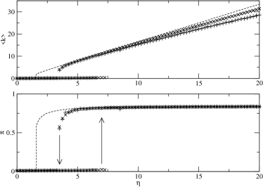
Figure 3: Mean degree $\left<k\right>$ (top) and probability that two randomly chosen nodes are within $\bar{d}$ of each other, $\pi$ (bottom), as a function of $\eta$. Shown are simulations with $n=200$ (plusses) and $n=500$ (crosses). Also theory for the high connected phase (dashed line). For large $\eta$, the data points converge towards the theory curve as $n$ increases. Arrows denote the approximate point at which the system jumps from one phase to the other. Here $\epsilon=0.001$, noise strength $\Delta=1$, similarity threshold $\bar{d}=2$. The system was run up to $t=1000$ for equilibration, then from $t=1000$ to $t=1100$ for data taking.

Fig. 3 shows that this model exhibits the same generic phenomenology of a sharp transition and the coexistence of sparse and dense network phases. The key consideration, in this case, is that when the link density is high, the distribution of $h_{i}$ in the population is narrow and hence link creation proceeds at a relatively fast rate.

This intuition is captured by a simple mean field approach. We will assume that the network can be well approximated by an Erdos-Renyi random graph with average degree $\langle{k}\rangle$. When $\nu\gg\eta,\lambda$, we can assume that the distribution of $h_{i}$ adjusts adiabatically to the changing network. In this limit the dynamics is well described by the Edwards-Wilkinson Langevin equation footnote3 .

$$\dot{h}_{i}=-\frac{\nu}{|{\cal N}_{i}|}\sum_{j\in{\cal N}_{i}}(h_{j}-h_{i})+\zeta_{i}\equiv-\nu\sum_{j}{\cal L}_{i,j}h_{j}+\zeta_{i}$$ (10)

This can be seen by considering a small time interval $dt$. If $\nu dt\gg 1$, the number of updates on each site is large and can be approximated with the central limit theorem with the two terms in Eq. (10). In this equation, $\zeta_{i}(t)$ is a white noise term with zero average and $\langle{\zeta_{i}(t)\zeta_{j}(t^{\prime})}\rangle=\nu^{2}\Delta\delta_{i,j}\delta(t-t^{\prime})$ and we have introduced the (normalized) Laplacian matrix of the graph ${\cal L}$. The dynamics of this model is easily integrated in the normal modes of the diffusion operator. In other words, let $\vec{v}^{\mu}$ be the eigenvectors of ${\cal L}$, i.e. ${\cal L}\vec{v}^{\mu}=\mu\vec{v}^{\mu}$, then the normal modes $h^{\mu}=\sum_{i}v_{i}^{\mu}h_{i}$ satisfy

$$\dot{h}^{\mu}=-\nu\mu h^{\mu}-\zeta^{\mu}$$ (11)

where, in view of the orthogonality of the transformation $i\to\mu$, $\zeta^{\mu}$ is again a white noise with the same statistical properties of $\zeta_{i}$. The fluctuations of $h^{\mu}$ in the stationary state are $\langle{(h^{\mu}-\langle{h^{\mu}}\rangle)^{2}}\rangle=\frac{\nu\Delta}{2\mu}$. Back transforming to the variables $h_{i}$ one finds that

$$\langle{(h_{i}-\langle{h_{i}}\rangle)^{2}}\rangle=\sum_{\mu>0}\frac{\nu\Delta}{2\mu}=\frac{\nu\Delta}{2}\int\frac{d\mu}{\mu}\rho(\mu)$$ (12)

where $\rho(\mu)$ is the density of eigenvalues of the Laplacian matrix, which has been computed in the limit $n\to\infty$ dgms_spectra . Notice that we disregard finite size clusters, which contribute to a $\mu=0$ peak in the spectrum, assuming that the $h_{i}$ value of these nodes is broadly distributed so that $d_{i,j}>\bar{d}$ whenever $i$ or $j$ are not in the giant component. There is no simple closed form for $\rho(\mu)$, so one has to resort to numerical calculation. To our level of approximation, it is sufficient to stick to a simple approximation dgms_spectra , where

$$\rho(\mu)=-{1\over\pi}\text{ Im }{1\over\mu-T(\mu)}.$$ (13)

and $T(\mu)$ is the solution of

$$T(\mu)={1\over\langle{k}\rangle}\sum_{k}{kP(k)\over k\mu+i\epsilon-(k-1)T(\mu)}$$ (14)

with $\epsilon\to 0^{+}$. The key features are that:

• the integral

  $$R(\langle{k}\rangle)=\int\frac{d\mu}{\mu}\rho(\mu)$$

  for Erdos-Renyi graphs, is a function of the average degree $\langle{k}\rangle$ alone.

• The function $R(c)$ decreases monotonically and it diverges as $c\to 1^{+}$, when the giant component vanishes

This allows us to estimate the probability

$$P\{|h_{i}-h_{j}|<\bar{d}\}=\theta(\langle{k}\rangle-1){\rm erf}\left[\bar{d}/\sqrt{2\nu\Delta R(\langle{k}\rangle)}\right]$$ (15)

where the $\theta$ function implies that this probability vanishes for disconnected graphs. Equating the link formation and removal rate, finally provides an equation for $\langle{k}\rangle$ which reads

$$\frac{\lambda}{2\eta}\langle{k}\rangle=\epsilon+(1-\epsilon)\theta(\langle{k}\rangle-1){\rm erf}\left[\bar{d}/\sqrt{2\nu\Delta R(\langle{k}\rangle)}\right].$$ (16)

Fig. 3 reports the numerical solution of this equation for the same parameters as in the simulations. This agreement is reasonably good in view of the approximations made. Again the mean field approach overestimates the size of the coexistence region. The mean-field calculation reproduces the main qualitative behavior, even though it (again) overestimates the size of the coexistence region.

The emergence of features (a)-(c) depends crucially on the divergence of $R(\langle{k}\rangle)$ on the average degree when $\langle{k}\rangle\approx 1$. This divergence gets smoothed when $\nu$ decreases, which suggests that the discontinuous transition should turn into a smooth crossover beyond a critical value $\nu_{c}$. This scenario, which is reminiscent of the behavior at the liquid-gas phase transition, is indeed confirmed by numerical simulations.

VI Coordinating in a changing world

We now consider a further specialisation of the general framework where link formation requires some form of coordination, synchronisation, or compatibility. For example, a profitable interaction may fail to occur if the two parties do not agree on where and when to meet, or if they do not speak the same languages, and/or adopt compatible technologies and standards. In addition, it may well be that shared social norms and codes enhance trust and thus are largely needed for fruitful interaction.

To account for these considerations, we endow each agent with an attribute $x_{i}$ which may take one of $q$ different values, $x_{i}\in\{1,2,\ldots,q\}$. $x_{i}$ describes the internal state of the agent, specifying e.g. its technological standard, language, or the social norms she adopts. The formation of a new link $ij$ requires that $i$ and $j$ display the same attribute, i.e. $x_{i}=x_{j}$. This is a particularisation of the general Eq. (1) with $d_{ij}=1-\delta_{x_{i},x_{j}}$ and $0<\bar{d}<1$. For simplicity we set $\epsilon=0$ since in the present formulation there is always a finite probability that two nodes display the same attribute and hence can link. We assume each agent revises its attribute at rate $\nu$, choosing $x_{i}$ dependent on its neighbours’ $x_{j}$s according to:

$$P\{x_{i}(t)=x\}=\frac{1}{Z}\exp\left[\beta\sum_{j:ij\in g(t)}\delta_{x,x_{j}(t)}\right]$$ (17)

where $\beta$ tunes the tendency of agents to conform with their neighbours and $Z$ provides the normalisation. This adjustment rule coincides with the Kawasaki dynamics, which is known to sample the equilibrium distribution of the Potts model of statistical physics Baxter with temperature $T=1/(k_{B}\beta)$. Eq. (17) has been used extensively, mainly for $q=2$, in the socio-economic literature as a discrete choice model Blume ; Durlauf ; Young .

This model describes a situation where agents are engaged in bilateral interactions which however require a degree of coordination among partners (i.e. $x_{i}=x_{j}$). The agents attempt to improve their situation both by coordinating their value of $x_{i}$ with that of neighbours and by searching for neighbours in their same state and linking with them. Link removal models decay of links, e.g. due to obsolescence considerations. The stochastic nature of the choice rule (17) captures a degree of volatility or un-modelled features on which the interaction depends (e.g. one might think that agent $i$ might have some advantage for choosing a given value of $x_{i}$ at a particular time). From the point of view of statistical physics, the presence of a non-zero “temperature” prevents the system from getting stuck in imperfect states. We will consider these effects in more detail below (see section VII and Fig. 8) when discussing the case $\beta\to\infty$ in greater detail.

This is another manifestation of our general idea that network-mediated contact favors inter-node similarity. As in Section V, we focus on the case where such a similarity-enhancing dynamics proceeds at a much faster rate than the network dynamics. That is, $\nu\gg\eta,\lambda$ so that, at any given $t$ where the network $g(t)$ is about to change, the attribute dynamics on the $x_{i}$ have relaxed to a stationary state. The statistics of this state are those of the Potts model on the graph $g(t)$. For random graphs of specified degree distribution $p(k)$, the necessary statistics of the Potts model can be found DGM ; EM and this makes an analytic approach to this model possible. We shall first discuss an approximate theory to the general case and then focus on a particular limit where the model can be solved exactly.

VI.1 Method of Solution

Again we rely on the random graph approximation where the network is completely specified by the degree distribution $p(k)$. Now however the probability of two nodes being in the same state ${\it if}$ they are both in the giant component depends on the magnetisation of the giant component. The master equation for a general node of degree $k$ is,

$$\dot{p}(k)= \lambda(k+1)p(k+1)+2\eta p(k-1)\pi(k-1)$$ (18)

$$-\lambda kp(k)-2\eta p(k)\pi(k)$$

where $\pi(k)$ is the probability that a node of degree $k$ is in the same state as a randomly chosen node. This crucially depends on whether the Potts spins are ordered or not. Indeed, for sufficiently high $\beta$ the equivalence between the different $q$ spin states is broken in the stationary state of the Potts model with temperature $1/(k_{B}\beta)$. This is signalled by a non-zero value of the magnetization

$$m=\frac{q\langle\delta_{x,1}\rangle-1}{q-1}$$ (19)

where the average is both on the nodes of the giant component and on the stationary distribution. Without loss of generality, we can assume that $x=1$ is the state which is selected and $m>0$ implies $\langle\delta_{x,1}\rangle>1/q$. Then it is easy to see that

$$\pi(k)={1\over q}+{q-1\over q}\gamma(1-u^{k})m(k)m$$ (20)

where $\gamma$, $u$ are defined in Eqs. (2,4) and $m(k)=(q\langle\delta_{x,1}|k\rangle-1)/(q-1)$. Note that $\pi(k)$ and $m(k)$ depend on $k$, more highly connected nodes being on average more coordinated/magnetised (see figure 4).

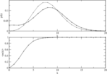
Figure 4: Results from the analytic solution. Upper plot: Plot of the degree distribution, $p(k)$ for $\eta/\lambda=4$, showing also the Poisson distribution with the same $\left<k\right>$ for comparison (dashed lines). Note that the degree distribution is not Poissonian. Lower plot: Plot of the average magnetisation of a node of degree $k$ for $\eta/\lambda=4$), showing that more highly connected nodes are, on average, more magnetised. $q=10$.

With these equations we can find $p(k)$ and $\pi(k)$ iteratively. Starting from a given $p(k)$, we first compute the properties of the Potts model on a random network with such a degree distribution, from which we get $\pi(k)$ in Eq. (20). This with Eq. (18) in the stationary state ($\dot{p}(k)=0$) allows us to estimate $x_{k}=p(k)/p(0)$ from the equation

$$x_{k+1}=\frac{[2\eta\pi(k)+\lambda k]x_{k}-2\eta\pi(k-\!1)x_{k-1}}{\lambda(k\!+\!1)}$$

iteratively, in terms of $x_{0}=1$ and $x_{1}=2\eta\pi(0)/\lambda$. Normalization, yields a new estimate of the degree distribution $p(k)=x_{k}/\sum_{h}x_{h}$. We repeat this cycle until a stable solution $p(k)$ is found.

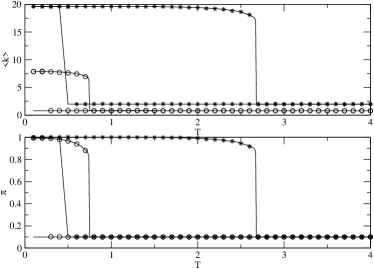
Figure 5: Upper plot: Plots of average degree ($\left<k\right>$) as a function of ’temperature’ $T=1/\beta$. Lower plot: Plots of the probability that two randomly chosen nodes are in the same state ($\pi$), as a function $1/\beta$. All plots are for: $\eta/\lambda=4$ (lower curves) and $\eta/\lambda=10$ (higher curves). Points are results of simulations. $q=10$. for $n=1000$.

Figure 5 shows $\left<k\right>$ and $\pi$ plotted against temperature for both simulations and theory. Note that the agreement is excellent despite the approximation made. As before, for high $\eta/\lambda$ there is a highly connected network with a giant component, for low $\eta/\lambda$ the network is sparsely connected. For intermediate values of $\eta/\lambda$ the two states coexist and which one is found depends on the initial conditions for $p(k)$.

Figure 6 shows a phase diagram (simulations and theory) for $\beta$ and $\eta/\lambda$. It can be seen that the theory is rather close to the simulation results. The low uncoordinated region is a Poisson random graph with $\left<k\right>=2\eta/(\lambda q)$. Starting in this state, the transition to the highly connected, magnetised state, can only occur when there is a giant component, i.e. $\left<k\right>>1$ so $\eta>\lambda q/2$. Hence the lowest point of the high connectivity region of figure 6 is at $\eta=5$ and $T=0$. Although $\nu\gg\eta,\lambda$, the simulations of the Potts model can still get into a metastable unmagnetised state, even below the transition temperature EM . The temperature $T$ at which this metastable state becomes unstable is given by EM

$$\exp(1/T)={\left<k^{2}\right>+(q-2)\left<k\right>\over\left<k^{2}\right>-2\left<k\right>}.$$ (21)

The (uncoordinated) graph is Poissonian, $\left<k^{2}\right>=\left<k\right>^{2}+\left<k\right>$. Thus the transition curve is

$$\eta_{c}={q\over 2}{\exp(1/T)+q-1\over\exp(1/T)-1}.$$ (22)

Monte-Carlo simulations show that this theoretical line is slowly approached as $n$ is increased.

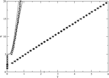
Figure 6: Phase diagram in $\eta$ ($\lambda=1$) and $T$, showing the high and low connectivity phases and the hysteretic region. Crosses are simulations ($n=5000,10000$), plusses are theory, the points are in pairs, one on each side of the phase line. The curves are theory, the leftmost curve is $\eta_{c}=(q/2)(\exp(1/T)+q-1)/(\exp(1/T)-1)$ which is the expected transition line if the system gets stuck in the metastable, unmagnetised state. The right curve is found using the normal method described above.
Upper left: higher connectivity, coordinated region.
Lower right: lower connectivity, uncoordinated region.
The central region is the hysteretic region.

VII Exact Solution for $T=0$.

The model with $\beta\to\infty$ and $\epsilon=0$ can be described exactly. We assume that in the initial state, links exist only between nodes that have the same spin, $\sigma_{i}=sigma_{j}$. The key intuition is that the spin of site $i$ can change only if $k_{i}=0$, i.e. if the site is isolated. Hence we can classify sites in disjoint subsets $N=N_{0}\bigcup_{\sigma=1}^{q}N_{\sigma}$ where

$$N_{0} =\{i:k_{i}=0\}$$

$$N_{\sigma} =\{i:k_{i}>0,\sigma_{i}=\sigma\}~{}~{}~{}~{}~{}\sigma=1,\ldots,q$$ (23)

The spins $\sigma_{i}$ are frozen for all nodes $i\in N_{\sigma}$ with $\sigma>0$ whereas nodes in $N_{0}$ have spin which are randomly updated at a fast rate. Because $\epsilon=0$, links can only be formed between nodes $i$ and $j$ which are either both in the same component $N_{\sigma}$ with $\sigma>0$, or both in $N_{0}$ provided they have the same spin, or if one is in $N_{\sigma}$ and one is in $N_{0}$, but has spin $\sigma_{j}=\sigma$. No link can be formed between $i\in N_{\sigma}$ and $j\in N_{\sigma^{\prime}}$ with $\sigma,\sigma^{\prime}>0$.

When a link with a node in $N_{0}$ is formed, one or two nodes pass from $N_{0}$ to some $N_{\sigma}$. Likewise nodes of $N_{\sigma}$ which lose their links move to $N_{0}$. Such a dynamics, in the limit $n\to\infty$ is captured by the following evolution for the fraction $n_{\sigma}$ of nodes in set $N_{\sigma}$ ($\sigma\geq 0$)

$$\dot{n}_{\sigma}={\frac{2\eta}{q}}n_{0}n_{\sigma}+{\frac{2\eta}{q^{2}}}n_{0}^{2}-\lambda p_{\sigma,1}n_{\sigma},~{}~{}~{}~{}\sigma\geq 1.$$ (24)

Here $p_{\sigma,k}$ is the degree distribution of nodes in $N_{\sigma}$, and

$$n_{0}=1-\sum_{\sigma=1}^{q}n_{\sigma}$$ (25)

is fixed by the normalization. The first term in Eq. (24) arises from the process where a node of degree zero joins a node of type $\sigma$. The factor 2 is present because either node might have initiated the link. The second term is the process where a node of degree zero joins another node of degree zero. The factor 2 is present because $n_{\sigma}$ increases by 2. The dynamics of the degree inside a component is just that leading to a random Poissonian graph for $k_{i}>0$. Hence $p_{\sigma,k}$ is given by

$$p_{\sigma,k}=\frac{c_{\sigma}^{k}}{(e^{c_{\sigma}}-1)k!},~{}~{}~{}~{}~{}k\geq 1$$ (26)

where the average degree

$$c_{\sigma}=\frac{2\eta n_{0}}{\lambda q}+\frac{2\eta n_{\sigma}}{\lambda}$$ (27)

is obtained by balancing the average link creation rate $2\eta(n_{\sigma}+n_{0}/q)$ with the link removal rate $\lambda c_{\sigma}$, inside the component $N_{\sigma}$. The equations above allow we to recast the dynamics in the form

$$\dot{n}_{\sigma}={\lambda^{2}c_{\sigma}\over 2\eta[1-\exp(-c_{\sigma})]}\left[{2\eta n_{0}\over\lambda q}-c_{\sigma}\exp(-c_{\sigma})\right].$$ (28)

From this it is clear that in the stationary states $c_{\sigma}$ obeys:

$$c_{\sigma}\exp(-c_{\sigma})={2\eta n_{0}\over\lambda q}$$ (29)

for $\sigma=1$ to $q$. Moreover Eq. (27) implies with the constraint

$$\sum_{\sigma=1}^{q}c_{\sigma}={2\eta\over\lambda}.$$ (30)

In order to build a solution, let us notice that Eq. (29) has two solutions (provided that $2\eta n_{0}\leq\lambda qe^{-1}$) which we denote $c_{+}>1$ and $c_{-}<1$. Hence solutions can be specified in terms of the number $\ell$ of components with $c_{\sigma}=c_{+}$. Then Eq. (30) becomes

$$\ell c_{+}+(q-\ell)c_{-}={2\eta\over\lambda}$$ (31)

Equations (29, 31) can be solved for any value of $\eta/\lambda$ and $\ell$.

The degree distribution for the whole network is given by:

$$p(k)={n_{0}\over q}\left[\ell{{c_{+}}^{k}\over k!}+(q-\ell){{c_{-}}^{k}\over k!}\right].$$ (32)

The average degree can be written as

$$\left<k\right>={\ell c_{+}^{2}+(q-\ell)c_{-}^{2}\over\ell c_{+}+(q-\ell)c_{-}}$$ (33)

We will now show that only the solutions with $\ell=0$ and $1$ are dynamically stable. These are those which describe the behavior of the model.

VII.1 Stability Analysis

The dynamics can be written as $\dot{n}_{\sigma}=f(n_{0},n_{\sigma})$. Let $n_{\sigma}={\bar{n}}_{\sigma}+\epsilon_{\sigma}$ where $\bar{n}_{\sigma}$ is the solution derived above (i.e. $f(\bar{n}_{\sigma},\bar{n}_{0})=0$) with $c_{\sigma}=c_{+}$ for $\sigma\leq\ell$ and $c_{\sigma}=c_{-}$ for $\sigma>\ell$. Here $\epsilon_{\sigma}$ is a small perturbation which, to leading order, satisfies

$$\dot{\epsilon}_{\sigma}={\lambda}\sum_{\nu=1}^{q}{T_{\sigma,\nu}}\epsilon_{\nu}$$ (34)

where ${\bf T}$ has matrix elements

$$T_{\sigma,\nu}={c_{\sigma}(c_{\sigma}-1)\over\exp(c_{\sigma})-1}\delta_{\sigma,\nu}-\frac{1}{q}\left[\frac{c_{\sigma}^{2}}{\exp(c_{\sigma})-1}+c_{\sigma}\right]$$ (35)

A solution is stable if all eigenvalues of ${\bf T}$ are negative. For the $\ell=0$ solution, $c_{\sigma}=c_{-}=2\eta/(\lambda q)$ for all $\sigma$, we find $q-1$ “transverse” eigenmodes ($\sum_{\sigma}\epsilon_{\sigma}=0$) with eigenvalue $\mu=-(1-c_{-})/(e^{c_{-}}-1)$ and one “longitudinal” mode ($\epsilon_{\sigma}=\epsilon$) with $\mu=-c_{-}/(1-e^{-c_{-}})$. Both are stable ($\mu<0$) so the $\ell=0$ solution is always stable, as long as $c_{-}<1$, i.e. for $2\eta<\lambda q$ (see Eq. 31).

It is also easy to find an unstable mode for solutions with $\ell\geq 2$ components in the $c_{+}$ state. Let $c_{\sigma}=c_{+}$ for $\sigma\leq\ell$ and $c_{\sigma}=c_{-}$ otherwise and consider “transverse” perturbations with $\epsilon_{\sigma}=0$ for $\sigma>\ell$ and $\sum_{\sigma}\epsilon_{\sigma}=0$. These describe density fluctuations among $c_{+}$ components. We find $\dot{\epsilon}_{\sigma}=\lambda\mu\epsilon$ with $\mu=c_{+}(c_{+}-1)/(e^{c_{+}}-1)>0$. This means that any perturbation of $\ell>1$ solutions with an imbalance between two or more components with $c_{\sigma}=c_{+}$ will grow exponentially, thus leading to the collapse of all but one of the components.

VII.2 The $\ell=1$ solution

Combining equations (29, 31), the equation for $c_{-}$ with $\ell=1$ can be written as

$$c_{-}-\frac{2\eta/\lambda-qc_{-}}{e^{2\eta/\lambda-qc_{-}}-1}=0.$$ (36)

This equation has no solution for $\eta<\eta_{c}$, where $\eta_{c}$ is the point where the maximum of the l.h.s. of Eq. (36) as a function of $c_{-}$, becomes zero. Beyond this point ($\eta>\eta_{c}$) two solutions appear. The one with larger value of $c_{-}$ merges with the $\ell=0$ solution, as $c_{-}\to 1$ when $\eta\to\lambda q/2$. This solution is un-physical as it describes a network where $c_{+}$, and hence the average degree, decreases with the networking effort $\eta$ (or with decreasing volatility $\lambda$). Indeed, a detailed analysis of the linear stability reveals the presence of an unstable mode footnote4 .

The lower branch instead has $c_{-}\to 0$ as $\eta\to\infty$ and it describes a physical solution with average degree increasing with $\eta/\lambda$. Numerical analysis of the stability matrix shows that this branch is indeed dynamically stable.

The critical point $\eta_{c}(q)$ at which the $\ell=1$ solution converges to $\lambda$ when $q\to 2$, which is the point where the $\ell=0$ solution ceases to exist. So the transition is continuous for $q=2$ and there is only one branch. For $q=10$ we find $\eta_{c}=2.27989...\lambda$ and for large $q$ we find $\eta_{c}\propto\log q$.

In summary, the system has either one or two stable states, depending on the values of $q$ and $\eta/\lambda$. For $\eta<\eta_{c}$ only the solution $\ell=0$ is stable, for $\eta>\lambda q/2$ only the solution $\ell=1$ is stable. Finally in the interval $\eta_{c}<\eta<\lambda q/2$ there are two stable solutions. The coexistence region $[\eta_{c},\lambda q/2]$ shrinks to a single point when $q=2$ and it gets larger as $q$ increases.

Figure 7 shows plots of $\left<k\right>$ against $\eta/\lambda$ for $q=10$ for both simulations and the theory described here.

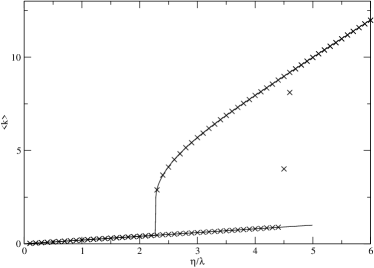
Figure 7: Plots of the mean connectivity $\left<k\right>$ as a function of $\eta/\lambda$. Lines are theory, crosses are simulations, $n=10000$, run to $t=100$ for equilibration, then to $t=200$ for data taking. For n=10000 the q=10 low state is unstable below the predicted value of 5 due to fluctuations being significant for finite n. The crosses that do not lie on the theory curves are systems which ’jumped’ during the data taking.

Concerning the degree distribution, it is worth noticing that the $\ell=0$ solution is characterized by a trivial Poisson distribution for the whole random graph. Since $\left<k\right>=c_{-}<1$, there is no giant component and the system is composed of many disconnected components of few nodes. The solution with $\ell=1$ is however non-trivial. In this case we have a network whose $p(k)$ is the sum of two Poisson distributions, one of which has $c_{+}>1$ and thus a giant component, whilst the other (consisting of $q-1$ separate networks plus the $k=0$ nodes) has $c_{-}<1$ and thus has no giant component.

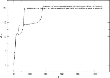
Figure 8: Plots of mean connectivity ${k}$ against time for networks starting in an initially unconnected state with $n=5000$ and $q=10$ and $\lambda=1$. The curve on the top right is $\eta=20$ and the other is $\eta=10$.

Even if $\ell>1$ states are unstable, they may occur in the early stages of the stochastic evolution of the network. Figure 8 shows time-series plots of simulations for relatively large $\eta$ ($\eta=10,20$), starting in an initially unconnected state. Although the $\eta=10$ solution eventually reaches its expected value of $\left<k\right>\cong 20$, its approach to that value is not smooth as might have been expected. Rather we find that the network spends some time in an intermediate $\ell>1$ metastable state. As we move to $\eta=20$, the time spent in metastable states increases substantially, failing to reach the stationary $\ell=1$ state (where $\left<k\right>\cong 40$) despite the relatively long simulation time. The reason for this behavior is that initially more than one giant component forms, with different values of $\sigma$. This state persists for a typical time $t_{\rm meta}$ which is inversely proportional to the eigenvalue of the unstable mode. Hence $t_{\rm meta}\sim 1/\mu\sim e^{c_{+}}\eta/(\lambda c_{+}^{2})$ becomes very long when $c_{+}$ is large. The reason why the dynamics is so slow depends on the fact that in order for nodes to migrate from one component $\sigma$ to another one, they have to loose all their links. Such a process is limited by the density $p_{\sigma,1}$ of nodes in component $\sigma$ with $k=1$, which is very small when $c_{+}$ is large ($p_{\sigma,1}\sim e^{-c_{\sigma}}$).

In such a situation introducing a stochastic element in agents’ choice (i.e. switching on $T>0$) or allowing for the formation of uncoordinated links (i.e. $\epsilon>0$) would make the system converge very fast to the coordinated state. In other words, this is a case where a finite “temperature” may allow the agents to find the global optimum more quickly and it might be rational for agents to resort to a stochastic choice rule. The ability to find an optimal state more quickly is also of advantage if there are external (exogenous) shocks which occasionally perturb the system.

VII.3 Discussion

The $T=0$ case is of particular interest because it can be solved exactly. For the other models described here, the coordination/correlation of the nodes were too complex for us to analyse exactly. In this section we have exactly solved a non-trivial network model. This was possible because of the fact that an agent only changes its spin if it has degree zero. The network is found to be the sum of $q$ Poissonian random graphs gecomment .

VIII Conclusion

In this paper we have proposed a general theoretical setup to study the dynamics of a social network that is flexible enough to admit a wide variety of particular specifications. We have studied three such specifications, each illustrating a distinct way in which the network dynamics may interact with the adjustment of node attributes. In all these cases, network evolution displays the three features (sharp transitions, resilience, and equilibrium co-existence) that empirical research has found to be common to many social-network phenomena. Our analysis indicates that these features arise as a consequence of the cumulative self-reinforcing effects induced by the interplay of two complementary considerations. On the one hand, there is the subprocess by which agent similarity is enhanced across linked (or close-by) agents. On the other hand, there is the fact that the formation of new links is much easier between similar agents. When such a feedback process is triggered, it provides a powerful mechanism that effectively offsets the link decay induced by volatility.

The similarity-based forces driving the dynamics of the model are at work in many socio-economic environments. Thus, even though fruitful economic interaction often requires that the agents involved display some “complementary diversity” in certain dimensions (e.g. buyers and sellers), a key prerequisite is also that agents can coordinate in a number of other dimensions (e.g. technological standards or trading conventions). Analogous considerations arise as well in the evolution of many other social phenomena (e.g. the burst of social pathologies discussed above) that, unlike what is claimed e.g. by Crane Crane , can hardly be understood as a process of epidemic contagion on a given network. It is by now well understood Bailey ; PV that such epidemic processes do not match the phenomenology reported in empirical research. Our model suggests that a satisfactory account of these phenomena must aim at integrating both the dynamics on the network with that of the network itself as part of a genuinely co-evolutionary process.

One common feature of all the models discussed in this paper is that stable states can have either a single giant component or none. Many real situations are characterized by stable states with a multitude of distinct components, barely connected. One example is the polarization of opinion (e.g. in politics) where the tendency of individuals to have opinions similar to those of the peers they interact with may also lead to the segregation of the population in different communities, of like mined individuals. The results presented here suggest that there must be a specific mechanism which is responsible for such a polarization. We hope that future work in this direction may shed some light on this issue.

- (1) D. J. Watts and S.H. Strogatz, Nature 393, 440-442 (1998).
- (2) L. K. Gallos, R. Cohen, P. Argyrakis, A. Bunde, and S. Havlin Phys. Rev. Lett. 94, 188701 (2005).
- (3) R Milo, S Shen-Orr, S Itzkovitz, N Kashtan, D Chklovskii and U Alon, Science, 298:824-827 (2002).
- (4) M. Granovetter, American Journal of Sociology 91, 481-510 (1985).
- (5) E. Glaeser, B. Sacerdote and J. Scheinkman, Quarterly Journal of Economics 111, 507-548 (1996).
- (6) D. L. Haynie, American Journal of Sociology 106, 1013-1057 (2001).
- (7) J. Crane, American Journal of Sociology 96, 1226-1259 (1991).
- (8) D.J. Harding, American Journal of Sociology 109, 676-719 (2003).
- (9) Organization for Economic Cooperation and Development, Networks of Enterprises and Local Development, OECD monograph (1996).
- (10) A. Saxenian, Regional Advantage: Culture and Competition in Silicon Valley and Route 128, Cambridge, Mass., Harvard University Press (1994).
- (11) E. J. Castilla, H. Hwang, E. Granovetter, and M. Granovetter: “Social Networks in Silicon Valley,” in C.-M. Lee, W. F. Miller, M. G. Hancock, and H. S. Rowen, editors, The Silicon Valley Edge, Stanford, Stanford University Press (2000).
- (12) M. Newman, Proceedings of the National Academy of Sciences 101, 5200-05 (2004).
- (13) S. Goyal, M.J. van der Leij, J.L. Moraga-González, FEEM Working Paper No. 84.04; Tinbergen Institute Discussion Paper No. 04-001/1 (2004).
- (14) J. Hagedoorn, Research Policy 31, 477-492 (2002).
- (15) B. Kogut, Strategic Management Journal 9, 319–332 (1988).
- (16) Y. Benkler, Yale Law Journal 112, 369-48 (2002).
- (17) Specifically, Hagerdon Hagedoorn reports that 99% of the R&D partnerships worldwide are conducted among firms in the so-called Triad: North America, Europe and Japan.
- (18) We recall that saying that a Poisson process occurs at a rate is equivalent to saying that it occurs with probability , independently, in any infinitesimal time interval .
- (19) M.E. Newman, S.H. Strogatz and D.J. Watts, Phys. Rev. E 64, 026118, (2001).
- (20) J. S. Coleman, American Journal of Sociology 94, S95-S120 (1988).
- (21) K. Annen, Journal of Economic Behavior and Organization 50, 449-63 (2003).
- (22) G. Bianconi, M. Marsili, F. Vega-Redondo, Physica A, 346, 116 (2005).
- (23) M. Marsili, F. Vega-Redondo and F. Slanina, Proceedings of the National Academy of Sciences, USA 101, 1439-43 (2004).
- (24) M. Granovetter, Getting a Job: A Study of Contacts and Careers. Chicago, Chicago University Press, 2nd. edition (1995).
- (25) G. Ehrhardt, M. Marsili and F. Vega-Redondo (2006), forthcoming in Int. J. Game. Theory.
- (26) T. Halpin-Healy and Y-C Zhang, Phys. Rep. 254, 215-415 (1995).
- (27) Weisbuch G, Deffuant G, Amblard F, Physica A 353 555-575 (2005).
- (28) S. N. Majumdar and P. L. Krapivsky, Phys. Rev. E 63, 045101 (2001).
- (29) DeMarzo, P., D. Vayanos, and J. Zwiebel (2003) Quarterly Journal of Economics 118, 909-968.
- (30) In order to derive such an equation, fix a small time interval . If the number of updates on each site will be large and hence, by the central limit theorem, the corresponding increments in the ’s are well approximated by a deterministic term equal to the expected value of the r.h.s. of Eq. (1), times , plus a random Gaussian contribution.
- (31) S.N. Dorogovtsev, A.V. Goltsev, J.F.F. Mendes and A.N. Samukhin, Phys. Rev. E 68 046109 (2003).
- (32) R.J. Baxter, Exactly Solved Models in Statistical Mechanics, London Academic Press (1982).
- (33) L. Blume, Games and Economic Behavior 4, 387-424 (1993).
- (34) S. Durlauf, Review of Economic Studies 60, 349-366 (1933).
- (35) P. Young, Individual Strategy and Social Structure: An Evolutionary Theory of Institutions, Princeton NJ, Princeton University Press (1998).
- (36) S.N. Dorogovtsev, A.V. Goltsev and J. Mendes, Eur. Phys. J. B 38, 177-182 (2004).
- (37) G.C.M.A. Ehrhardt and M. Marsili, J. Stat. Mech. (2005) P02006.
- (38) In this case there are eigenmodes describing mass transfer across components (i.e. ) and two eigenmodes with and for . One of these is unstable.
- (39) The fact that the sub-graphs are Poissonian (that they are fully specified by their degree distribution) is linked to the fact that we could find an exact solution.
- (40) N.T.J. Bailey, The Mathematical Theory of Infectious Diseases and Its Applications, New York, Hafner Press (1975).
- (41) R. Pastor-Satorras and A. Vespignani, Phys. Rev. Lett. 86, 3200-3203 (2001).