On the Solution of Maxwell’s First
Order Equations

Max-Planck-Institut für Plasmaphysik, D-85741 Garching, Germany

Abstract

In an attempt to solve Maxwell’s first order system of equations, starting from a given initial state, it is found that a consistent solution depending on the temporal evolution of the sources cannot be calculated. The well known retarded solutions of the second order equations, which are based on the introduction of potentials, turn out to be in disagreement with a direct solution of the first order system.
PACS number: 03.50.De

1. Introduction

In recent papers [1, 2] it was shown that Maxwell’s equations have different formal solutions depending on the chosen gauge. In [2] it was argued that the formalism of gauge invariance is based on the tacit assumption of Maxwell’s equations having unique solutions which appeared, however, not to be guaranteed a priori. In response to the publication of [2] it was pointed out in private communications [3] that uniqueness is a necessary consequence of the linear structure of the equations. These arguments are valid. If one finds, nevertheless, different solutions in Lorenz and in Coulomb gauge, it seems to indicate that a solution does not exist at all. Indeed, it was shown in [2] that the Liénard-Wiechert fields based on the Lorenz gauge do not satisfy the equations in the source region, unless one postulates a velocity dependent “deformation” of point charges as in [1]. Furthermore, the formal solution for the vector potential in Coulomb gauge led to an undefined conditionally convergent integral which would even diverge upon differentiation.

The reason for the difficulties encountered could have to do with the assumption of point sources which were exclusively considered in [2]. Therefore, it appears worthwhile to investigate the problem further, assuming smooth charge and current distributions as originally considered by Maxwell. In order to avoid any ambiguities arising from the introduction of potentials, it seems advisable to analyse directly the solvability of the first order system of Maxwell’s equations (Sect. 2.). It turns out that the coupled first order system contains certain inconsistencies which prevent its solution when calculated by a numerical forward method proceeding in time.

The usual method of solution derives inhomogeneous wave equations from the first order system, and expresses the solutions as retarded integrals by application of Duhamel’s principle. In [2] it was argued that this method is not plausible, since the wave equations obtained by differentiating the first order system connect the travelling fields with the stationary sources at the same time, while in the retarded solutions the differentiation of the sources is inconsistently dated back to an earlier time. In Sect. 3. we analyze the retarded solutions for smooth source distributions and find that these solutions do not satisfy the first order system. This is demonstrated in Sect. 4. by considering a specific example.

2. The first order equations

In vacuo the first order system as devised by Hertz on the basis of Maxwell’s equations is supposed to describe the electromagnetic field:

$$div\,\vec{E}_{g}=4\pi\,\rho$$ (1)

$$rot\,\vec{E}_{r}=-\frac{1}{c}\frac{\partial\vec{B}}{\partial t}$$ (2)

$$div\,\vec{B}=0$$ (3)

$$rot\,\vec{B}=\frac{4\pi}{c}\,\vec{j}+\frac{1}{c}\frac{\partial\left({\vec{E}_{g}+\vec{E}_{r}}\right)}{\partial t}$$ (4)

Here we have indicated that the electric field has two contributions of different structure. In (1) only the irrotational part enters, whereas (2) contains exclusively the rotational part of the field. Both parts enter equation (4). One may separate out the instantaneous contribution of the magnetic field and write (4) as two equations:

$$rot\,\vec{B}_{0}=\frac{4\pi}{c}\,\vec{j}+\frac{1}{c}\frac{\partial\vec{E}_{g}}{\partial t}$$ (5)

$$rot\,\vec{B}_{1}=\frac{1}{c}\frac{\partial\vec{E}_{r}}{\partial t}$$ (6)

The quasi-static solutions of (1) and (5) – subject to the boundary condition that the fields vanish at infinity – are represented by integrals over all space:

$$\vec{E}_{g}\left({\vec{x},\,t}\right)=\int\!\!\!\int\!\!\!\int{\rho\left({\vec{x}^{\prime},\,t}\right)}\,\left({\vec{x}-\vec{x}^{\prime}}\right)\frac{d^{3}x^{\prime}}{\left|{\vec{x}-\vec{x}^{\prime}}\right|^{3}}$$ (7)

$$\vec{B}_{0}\left({\vec{x},\,t}\right)=\frac{1}{c}\int\!\!\!\int\!\!\!\int{\left({\vec{j}\left({\vec{x}^{\prime},\,t}\right)+\frac{1}{4\pi}\frac{\partial\vec{E}_{g}\left({\vec{x}^{\prime},\,t}\right)}{\partial t}}\right)}\times\left({\vec{x}-\vec{x}^{\prime}}\right)\,\frac{d^{3}x^{\prime}}{\left|{\vec{x}-\vec{x}^{\prime}}\right|^{3}}$$ (8)

It remains then to determine the rotational part of the electric field and the contribution $\vec{B}_{1}$.

Applying a numerical forward method one obtains from (6) the difference equation:

$$\vec{E}_{r}\left({\Delta t}\right)=\vec{E}_{r}\left(0\right)+\Delta t\,c\,rot\,\vec{B}_{1}\left(0\right)$$ (9)

and from (2):

$$\vec{B}\left({\Delta t}\right)=\vec{B}\left(0\right)-\Delta t\,c\,rot\,\vec{E}_{r}\left(0\right)$$ (10)

Assuming that the sources were constant for $t\leq 0$ one has the initial conditions:

$$\vec{E}_{r}\left(0\right)=\vec{B}_{1}\left(0\right)=0$$ (11)

Substituting this into (9) and (10) one finds the curious result that neither $\vec{E}_{r}$ nor the total magnetic field $\vec{B}$ proceed after the first time step, and this will remain so forever, at least in the vacuum region outside the sources. If the current would linearly rise to a new stationary level, e.g., equation (10) would predict that $\vec{B}$ stays constant at its initial value, in contrast to (8) which predicts that $\vec{B}_{0}$ rises simultaneously with the current and reaches a new stationary value as well.

One may also split (2) into two equations:

$$rot\,\vec{E}_{r0}=-\frac{1}{c}\frac{\partial\vec{B}_{0}}{\partial t}$$ (12)

$$rot\,\vec{E}_{r1}=-\frac{1}{c}\frac{\partial\vec{B}_{1}}{\partial t}$$ (13)

The quasi-static solution of (12) is:

$$\vec{E}_{r0}=-\frac{1}{4\pi\,c}\int\!\!\!\int\!\!\!\int{\frac{\partial\vec{B}_{0}}{\partial t}\times\frac{\vec{x}-\vec{x}^{\prime}}{\left|{\vec{x}-\vec{x}^{\prime}}\right|^{3}}}\,d^{3}x^{\prime}$$ (14)

and from (13) follows:

$$\vec{B}_{1}\left({\Delta t}\right)=\vec{B}_{1}\left(0\right)-\Delta t\,c\,rot\,\vec{E}_{r1}\left(0\right)=0$$ (15)

If $\vec{B}_{1}$ vanishes after the first time step as follows from (15), and $\vec{B}$ stays also constant according to (10), a clear contradiction with (8) arises. Furthermore, equation (9) predicts that the total rotational electric field stays constant, whereas the quasi-static part (14) follows instantaneously all changes of $\vec{B}_{0}\left(t\right)$ according to (14).

We note that the quasi-static expressions (7), (8), (14) can be seen as solutions of elliptic equations. On the other hand, one obtains from (2) and (4) by mutual elimination of the fields the inhomogeneous hyperbolic equations:

$$\Delta\vec{B}-\frac{1}{c^{2}}\frac{\partial^{2}\vec{B}}{\partial t^{2}}=-\frac{4\pi}{c}\,rot\,\vec{j}$$ (16)

$$\Delta\vec{E}_{r}-\frac{1}{c^{2}}\frac{\partial^{2}\vec{E}_{r}}{\partial t^{2}}=-\frac{4\pi}{c}\frac{\partial\vec{j}}{\partial t}\,+\frac{1}{c^{2}}\frac{\partial^{2}\vec{E}_{g}}{\partial t^{2}}\,$$ (17)

As indicated in [2], the mixture of elliptic and hyperbolic equations inherent to Maxwell’s system leads apparently to the inconsistencies which manifest themselves in the incongruities implied in (10) as compared to (8), and in (14) as compared to (9). The system (1 – 4) does not permit a continuous temporal evolution from a given realistic initial state. In a region where the sources in (16) and (17) vanish the homogeneous hyperbolic equations describe correctly propagating electromagnetic fields, but their production mechanism in connection to the sources remains obscure.

Since in all textbooks it is claimed that Maxwell’s equations do have solutions which are uniquely determined when the behaviour of the sources is given as a function of space and time, we must discuss the usual procedure to obtain these solutions which – according to our analysis – cannot satisfy the first order system.

3. The retarded solutions

The normal method of solution expresses the fields by potentials:

$$\vec{B}=rot\,\vec{A}\;,\quad\vec{E}=-\nabla\phi-\frac{1}{c}\frac{\partial\vec{A}}{\partial t}$$ (18)

which leads to inhomogeneous wave equations in Lorenz gauge:

$$\Delta\phi-\frac{1}{c^{2}}\frac{\partial^{2}\phi}{\partial t^{2}}=-4\pi\,\rho$$ (19)

$$\Delta\vec{A}-\frac{1}{c^{2}}\frac{\partial^{2}\vec{A}}{\partial t^{2}}=-\frac{4\pi}{c}\,\,\vec{j}$$ (20)

They are solved by application of Duhamel’s principle to yield the retarded solutions, e.g.:

$$\vec{A}\left({\vec{x}{\kern 1.0pt},\,t}\right)=\frac{1}{c}\int\!\!\!\int\!\!\!\int{\vec{j}}\left({\vec{x}^{\prime}{\kern 1.0pt},\,t-{\left|{\vec{x}{\kern 1.0pt}-\vec{x}^{\prime}{\kern 1.0pt}}\right|}\mathord{\left/{\vphantom{{\left|{\vec{x}{\kern 1.0pt}-\vec{x}^{\prime}{\kern 1.0pt}}\right|}c}}\right.\kern-1.2pt}c}\right)\,\frac{d^{3}x^{\prime}}{\left|{\vec{x}{\kern 1.0pt}-\vec{x}^{\prime}{\kern 1.0pt}}\right|}\,\,$$ (21)

Instead of introducing potentials one may solve the wave equations for the fields directly. The magnetic field, for example, can be expressed as the sum:

$$\vec{B}=\vec{B}_{0}+\vec{B}_{1}$$ (22)

where $\vec{B}_{0}$ is the instantaneous part (8), and $\vec{B}_{1}$ satisfies according to (16) the equation:

$$\Delta\vec{B}_{1}-\frac{1}{c^{2}}\frac{\partial^{2}\vec{B}_{1}}{\partial t^{2}}=\frac{1}{c^{2}}\frac{\partial^{2}\vec{B}_{0}}{\partial t^{2}}$$ (23)

In analogy to (21) this equation has the retarded solution:

$$\vec{B}_{1}\left({\vec{x}{\kern 1.0pt},\,t}\right)=-\frac{1}{4\pi\,c^{2}}\int\!\!\!\int\!\!\!\int{\left({\frac{\partial^{2}\vec{B}_{0}\left({\vec{x}^{\prime},\,t^{\prime}}\right)}{\partial t^{\prime 2}}}\right)}\,\frac{d^{3}x^{\prime}}{\left|{\vec{x}{\kern 1.0pt}-\vec{x}^{\prime}{\kern 1.0pt}}\right|}\;,\quad t^{\prime}=t-{\left|{\vec{x}{\kern 1.0pt}-\vec{x}^{\prime}{\kern 1.0pt}}\right|}\mathord{\left/{\vphantom{{\left|{\vec{x}{\kern 1.0pt}-\vec{x}^{\prime}{\kern 1.0pt}}\right|}c}}\right.\kern-1.2pt}c$$ (24)

Similarly, one may write:

$$\vec{E}=\vec{E}_{0}+\vec{E}_{1}$$ (25)

and obtain from (17) a second order differential equation for $\vec{E}_{1}$:

$$\Delta\vec{E}_{1}-\frac{1}{c^{2}}\frac{\partial^{2}\vec{E}_{1}}{\partial t^{2}}=\frac{1}{c^{2}}\frac{\partial^{2}\vec{E}_{0}}{\partial t^{2}}\,$$ (26)

where $\vec{E}_{0}$ is the instantaneous part of the electric field resulting from (5) and (12):

$$\vec{E}_{0}\left({\vec{x}{\kern 1.0pt},\,t}\right)=-\frac{1}{c^{2}}\int\!\!\!\int\!\!\!\int{\left({\frac{\partial\vec{j}\left({\vec{x}^{\prime},\,t}\right)}{\partial t}}\right)}\,\frac{d^{3}x^{\prime}}{\left|{\vec{x}{\kern 1.0pt}-\vec{x}^{\prime}{\kern 1.0pt}}\right|}$$ (27)

The retarded solution of (26) is then:

$$\vec{E}_{1}\left({\vec{x}{\kern 1.0pt},\,t}\right)=-\frac{1}{4\pi\,c^{2}}\int\!\!\!\int\!\!\!\int{\left({\frac{\partial^{2}\vec{E}_{0}\left({\vec{x}^{\prime},\,t^{\prime}}\right)}{\partial t^{\prime 2}}}\right)}\,\frac{d^{3}x^{\prime}}{\left|{\vec{x}{\kern 1.0pt}-\vec{x}^{\prime}{\kern 1.0pt}}\right|}\;,\quad t^{\prime}=t-{\left|{\vec{x}{\kern 1.0pt}-\vec{x}^{\prime}{\kern 1.0pt}}\right|}\mathord{\left/{\vphantom{{\left|{\vec{x}{\kern 1.0pt}-\vec{x}^{\prime}{\kern 1.0pt}}\right|}c}}\right.\kern-1.2pt}c$$ (28)

It turns out that the fields as obtained from (21) and (18) are not the same fields as that calculated from (22), (8), and (24), and from (25), (27), and (28). This will be demonstrated in the next Section by choosing a specific example. Hence, we must conclude that the retarded solutions cannot be considered as true solutions of the first order equations.

The reason for this failure must be sought in the inconsistency which lies in the fact that equations (20), (23), (26) connect the sources $\vec{j}\left({\vec{x}{\kern 1.0pt},t}\right)$, $\vec{B}_{0}\left({\vec{x}{\kern 1.0pt},t}\right)$, $\vec{E}_{0}\left({\vec{x}{\kern 1.0pt},t}\right)$, respectively, with the travelling wave fields $\vec{A}\left({\vec{x}{\kern 1.0pt},t}\right)$, $\vec{B}_{1}\left({\vec{x}{\kern 1.0pt},t}\right)$, $\vec{E}_{1}\left({\vec{x}{\kern 1.0pt},t}\right)$ at the same time $t$, whereas in the retarded solutions (21), (24), (28) the differentiation of the source is dated back to the earlier time $t^{\prime}=t-{\left|{\vec{x}{\kern 1.0pt}-\vec{x}^{\prime}{\kern 1.0pt}}\right|}\mathord{\left/{\vphantom{{\left|{\vec{x}{\kern 1.0pt}-\vec{x}^{\prime}{\kern 1.0pt}}\right|}c}}\right.\kern-1.2pt}c$. As pointed out in [2], the source may be very far away from the observation point, and may not even exist anymore when the fields $\vec{B}_{1}\left({\vec{x}{\kern 1.0pt},t}\right)$, $\vec{E}_{1}\left({\vec{x}{\kern 1.0pt},t}\right)$ are measured at time $t$. It makes little sense to differentiate non-existent instantaneous fields at time $t$, but this was necessary to derive equations (16), (17) from the system (1 – 4). Obviously, it constitutes a contradictio in adjecto connecting the travelling fields predicted by (16) and (17) with the stationary sources in the first order system at the same time.

4. A specific example

In order to facilitate the calculations we choose an example where we have $div\,\vec{j}=0$. In this case the scalar potential vanishes because of $\rho=0$ which makes Lorenz and Coulomb gauge identical: $div\,\vec{A}=0$. The chosen example is a hollow cylinder which carries a closed oscillating current driven by an rf-generator through a resistor R, as sketched in Fig. 1. It is assumed that the current was switched on at time $t=-\infty$ and oscillates with a sinusoidal time dependence: $I\,\exp\left({-i\,\omega\,t}\right)$. The current flows in a thin central filament, and returns symmetrically on the cylindrical surface. This can be achieved to an arbitrary degree of accuracy, if the inverse wave vector $k=\omega\mathord{\left/{\vphantom{\omega c}}\right.\kern-1.2pt}c$ is large compared to the dimensions of the device.

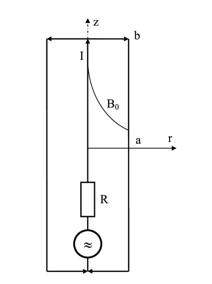
Figure 1: Oscillating current flowing in a closed circuit of cylindrical geometry

The instantaneous magnetic field component (8) produced in this configuration is:

$$B_{0} = \frac{2\,I}{c\,r}\exp\left({-i{\kern 1.0pt}\omega{\kern 1.0pt}t}\right)\;,\quad r\leq a\;,\quad-b\leq z\leq b$$ (29)

$$B_{0} = 0\;,\quad r>a\;,\quad z<-b\;,\quad z>b$$

and the instantaneous electric field (27) becomes:

$$\vec{E}_{0}=\frac{i\,k\,I}{2\pi\,c}\,\exp\left({-i{\kern 1.0pt}\omega{\kern 1.0pt}t}\right)\int\limits_{0}^{2\pi}{\left\{{\int\limits_{0}^{a}{\left[{\frac{\cos\varphi^{\prime}\,dr^{\prime}}{R}}\right]_{z^{\prime}=-b}^{z^{\prime}=+b}\,\vec{e}_{r}+\int\limits_{-b}^{b}{\left[{\frac{dz^{\prime}}{R}}\right]_{r^{\prime}=a}^{r^{\prime}=0}\vec{e}_{z}}}}\right\}}\,d\varphi^{\prime}$$ (30)

$$R=\sqrt{r^{2}+r^{\prime 2}-2\,r\,r^{\prime}\cos\varphi^{\prime}+\left({z-z^{\prime}}\right)^{2}}$$

The retarded solution of the vector potential as obtained from (21) is:

$$\vec{A}=\frac{I\,e^{-i{\kern 1.0pt}\omega{\kern 1.0pt}t}}{2\pi\,c}\int\limits_{0}^{2\pi}{\left\{{\int\limits_{0}^{a}{\left[{\frac{\exp\left({i\,k\,R}\right)}{R}}\right]}_{z^{\prime}=-b}^{z^{\prime}=+b}\cos\varphi^{\prime}\,dr^{\prime}\,\vec{e}_{r}+\int\limits_{-b}^{+b}{\left[{\frac{\exp\left({i\,k\,R}\right)}{R}}\right]_{r^{\prime}=a}^{r^{\prime}=0}dz^{\prime}\,\vec{e}_{z}}}\right\}}\,d\varphi^{\prime}$$ (31)

It may be substituted into (18) to yield the fields as given by Jackson for a localized oscillating source [4]:

$$B\!\! = \!\!\frac{I\,e^{-i{\kern 1.0pt}\omega{\kern 1.0pt}t}}{2\pi\,c}\int\limits_{0}^{2\pi}\left\{\int\limits_{0}^{a}{\left[{\frac{e^{i\,k\,R}\left({1-i\,k\,R}\right)\,s\,\cos\varphi^{\prime}dr^{\prime}}{R^{3}}}\right]_{s=z-b}^{s=z+b}}\right.$$ (32)

$$\quad\quad\quad\left.-\int\limits_{z-b}^{z+b}{\left[{\frac{e^{i\,k\,R}\left({1-i\,k\,R}\right)\,\left({r-r^{\prime}\cos\varphi^{\prime}}\right)\,dz^{\prime}}{R^{3}}}\right]_{r^{\prime}=0}^{r^{\prime}=a}}\right\}\,d\varphi^{\prime}$$

$$\vec{E}=\frac{i\,k\,I\,e^{-i{\kern 1.0pt}\omega{\kern 1.0pt}t}}{2\pi\,c}\int\limits_{0}^{2\pi}{\left\{{\int\limits_{0}^{a}{\left[{\frac{e^{i\,k\,R}\cos\varphi^{\prime}\,dr^{\prime}}{R}}\right]_{z^{\prime}=-b}^{z^{\prime}=+b}\,\vec{e}_{r}+\int\limits_{-b}^{b}{\left[{\frac{e^{i\,k\,R}\,dz^{\prime}}{R}}\right]_{r^{\prime}=a}^{r^{\prime}=0}\vec{e}_{z}}}}\right\}}\,d\varphi^{\prime}$$ (33)

where $s=z-z^{\prime}$. It is doubtful whether these solutions satisfy also the differential equations (23) and (26). In order to check on this we consider, e.g., equation (23) adapted to our case:

$$r^{2}\frac{\partial^{2}B_{1}}{\partial r^{2}}+r\,\frac{\partial B_{1}}{\partial r}-B_{1}\left({1-r^{2}k^{2}}\right)+r^{2}\frac{\partial^{2}B_{1}}{\partial z^{2}}=-\frac{2\,k^{2}I\,r}{c}\,e^{-i\,\omega\,t}$$ (34)

where the right-hand-side must be set to zero outside the cylinder of Fig. 1. We integrate this equation with respect to $r$ and obtain:

$$\frac{\partial B_{1}}{\partial r}-\frac{B_{1}}{r}+\frac{1}{r^{2}}\int\limits_{0}^{r}{r^{2}}\left({\frac{\partial^{2}B_{1}}{\partial z^{2}}+k^{2}B_{1}}\right)\,dr=-\frac{\,k^{2}I}{c}\,e^{-i\,\omega\,t}$$ (35)

The contribution $B_{1}$ may be calculated from (32) by expansion of the exponential function for $k\,R<1$. In zero order one obtains the instantaneous field (29), and in second order one has:

$$B_{1}=-\frac{I\,k^{2}e^{-i{\kern 1.0pt}\omega{\kern 1.0pt}t}}{4\pi\,c}\int\limits_{0}^{2\pi}{\left\{{\int\limits_{0}^{a}{\left[{\frac{s\cos\varphi^{\prime}dr^{\prime}}{R}}\right]_{s=z-b}^{s=z+b}\!\!\!\!-\int\limits_{z-b}^{z+b}{\left[{\frac{\left({r-r^{\prime}\cos\varphi^{\prime}}\right)\,dz^{\prime}}{R}}\right]_{r^{\prime}=0}^{r^{\prime}=a}}}}\right\}d\varphi^{\prime}}+O\left({k^{n>2}}\right)$$ (36)

The integration over $r^{\prime}$ and $z^{\prime}$ may be carried out analytically to yield:

$$B_{1}=\frac{I\,k^{2}e^{-i{\kern 1.0pt}\omega{\kern 1.0pt}t}}{4\pi\,c}\int\limits_{0}^{2\pi}{\left[{s\cos\varphi^{\prime}\ln\left({r^{\prime}-r\cos\varphi^{\prime}+R}\right)+\left({r-r^{\prime}\cos\varphi^{\prime}}\right)\ln\left({s+R}\right)}\right]_{s=z-b,\,r^{\prime}=0}^{s=z+b,\,r^{\prime}=a}d\varphi^{\prime}}$$ (37)

Expanding this expression in a power series of $r$, and inserting it into the left-hand-side of (34) we find for $z=0$:

$$\frac{I\,k^{2}e^{-i{\kern 1.0pt}\omega{\kern 1.0pt}t}}{2\,c}\,\left[{\left({\frac{b}{\left({a^{2}+b^{2}}\right)^{\frac{3}{2}}}-\frac{1}{b^{2}}}\right)\,r^{2}+\left({\frac{1}{2\,b^{4}}-\frac{b\left({2b^{2}-3a^{2}}\right)}{4\left({a^{2}+b^{2}}\right)^{\frac{7}{2}}}}\right)\,r^{4}}\right]\;+O\left({r^{n>4}}\right)$$ (38)

which is obviously at variance with the right-hand-side of (35). A similar conclusion is reached, if (33) is substituted into (26). This can only be checked numerically, since the instantaneous field $\vec{E}_{0}$ does not vanish outside the cylinder, in contrast to $\vec{B}_{0}$.

Result (38) proves that the standard solutions (32) and (33) do not satisfy the first order system from which equations (16) and (17) were derived. Hence, our conclusion in Sect. 2., namely that the first order system does not permit a solution, cannot be refuted by referring to the retarded solutions as taught in the textbooks such as [4].

There is also a physical reason to reject Jackson’s solution (31) for the considered case. If one calculates the fields with (18) from (31) and evaluates the Poynting vector $\vec{E}\times\vec{B}$ at large distance, one can integrate the total radiation power emitted by the closed circuit of Fig. 1:

$$P_{tot}=\int\!\!\!\int{\frac{c}{4\pi}}\left({\vec{E}\times\vec{B}}\right)\cdot\vec{d}^{2}x=\frac{I^{2}\,a^{4}\,b^{2}\,k^{6}}{6\,c}$$ (39)

This result is obviously not physical. The device in question may be seen as a short-circuited cable which should not continuously loose energy to the outside world; in particular not when the enclosing shell would be made out of superconducting material. The predicted power loss (39) could certainly not be confirmed experimentally.

5. Conclusions

It has been shown that an attempt to calculate numerically the temporal evolution of the electromagnetic field from the full set of Maxwell’s first order equations will fail due to the internal inconsistencies built into the coupled system of equations. As noted earlier [2], the reason lies in the fact that the travelling wave fields are connected with the stationary sources at the same time.

Maxwell’s equations describe correctly the production of the instantaneous electromagnetic field, and also the propagation of wave fields in empty space. The production mechanism of electromagnetic waves by time varying sources, however, does not find an explanation in the framework of Maxwell’s theory. Contrary to what is commonly believed, the retarded solutions for the electromagnetic potentials do not lead to fields which are in agreement with a direct solution of the second order differential equations for the fields.

Acknowledgment

The author is indebted to V. Onoochin for initiating this work. Vladimir contributed significantly in the early discussions, but he modestly felt that he should not be a co-author of the paper.

References

• [1] Onoochin V V 2002 Annales de la Fondation Louis de Broglie 27 163
• [2] Engelhardt W 2005 Annales de la Fondation Louis de Broglie 30 157
• [3] Prof. Daniele Funaro (University of Modena), Prof. Michel de Haan (Free University of Brussels), private communications
• [4] Jackson J D 1975 Classical Electrodynamics, Second Edition (New York: John Wiley & Sons, Inc), Sect. 9.1