Development of a BEM Solver using Exact Expressions for Computing the Influence of Singularity Distributions

Abstract

Closed form expressions for three-dimensional potential and force field due to singularities distributed on a finite flat surface have been used to develop a fast and accurate BEM solver. The exact expressions have been investigated in detail and found to be valid throughout the complete physical domain. Thus, it has been possible to precisely simulate the complicated characteristics of the potential and force field in the near-field domain. The BEM solver has been used to compute the capacitance of a unit square plate and a unit cube. The obtained values have compared well with very accurate values of the capacitances available in the literature.

1 Introduction

The boundary element method is based on the numerical implementation of boundary integral equations based on the Green’s formula. In order to carry out the implementation, the boundaries are generally segmented, and these boundary elements are endowed with distribution of singularities such as source, sink, dipoles and vortices. The singularity strengths are obtained through the satisfaction of boundary conditions (Dirichlet, Neumann or Robin) which calls for the computation of the influence of the singularities at the points where the boundary conditions are being satisfied. Once the singularity strengths are known, physical properties at any point within the physical domain can be easily estimated. Thus, accurate computation of the influence at a point in the domain of interest due to singularities distributed on a surface is of crucial importance.

In this work, we have presented a BEM solver based on closed form expressions of potential and force field due to a uniform distribution of source on a flat surface. In order to validate the expressions, the potential and force field in the near-field domain have been thoroughly investigated. In the process, the sharp changes and discontinuities which characterize the near-field domain have been easily reproduced. Since the expressions are analytic and valid for the complete physical domain, and no approximations regarding the size or shape of the singular surface have been made during their derivation, their application is not limited by the proximity of other singular surfaces or their curvature. Moreover, since both potential and force fields are evaluated using exact expressions, boundary conditions of any type, namely, Dirichlet (potential), Neumann (gradient of potential) or Robin (mixed) can be seamlessly handled.

As an application of the new solver, we have computed the capacitances of a unit square plate and a unit cube to very high precision. These problems have been considered to be two major unsolved problems of the electrostatic theory [Maxwell]-[Mascagni]. The capacitance values estimated by the present method have been compared with very accurate results available in the literature (using BEM and other methods). The comparison testifies to the accuracy of the approach and the developed solver.

2 Theory

The expression for potential (V) at a point $(X,Y,Z)$ in free space due to uniform source distributed on a rectangular flat surface having corners situated at $(x_{1},z_{1})$ and $(x_{2},z_{2})$ can be shown to be a multiple of

$$V(X,Y,Z)=\int_{z_{1}}^{z_{2}}\int_{x_{1}}^{x_{2}}\frac{dx\,dz}{\sqrt{(X-x)^{2}+Y^{2}+(Z-z)^{2}}}$$ (1)

where the value of the multiple depends upon the strength of the source and other physical considerations. Here, it has been assumed that the origin of the coordinate system lies on the surface plane ($XZ$). The closed form expression for $V(X,Y,Z)$ is as follows:

$$V(X,Y,Z)=$$ (2)

$$\frac{1}{2}\times$$

$$\left(\right.+2\,Z\,\ln\left(\frac{D_{2}\,-\,(X-x_{1})}{D_{1}\,-\,(X-x_{1})}\right)+2\,Z\,\ln\left(\frac{D_{3}\,-\,(X-x_{2})}{D_{4}\,-\,(X-x_{2})}\right)$$

$$+2\,x_{1}\,\ln\left(\frac{D_{1}\,-\,(Z-z_{1})}{D_{2}\,-\,(Z-z_{2})}\right)+2\,x_{2}\,\ln\left(\frac{D_{4}\,-\,(Z-z_{2})}{D_{3}\,-\,(Z-z_{1})}\right)$$

$$+2\,z_{1}\,\ln\left(\frac{D_{1}\,-\,(X-x_{1})}{D_{3}\,-\,(X-x_{2})}\right)+2\,z_{2}\,\ln\left(\frac{D_{4}\,-\,(X-x_{2})}{D_{2}\,-\,(X-x_{1})}\right)$$

$$-\,S_{1}\,\left(X\,+\,i\,\left|Y\right|\right)\,tanh^{-1}\left(\frac{R_{1}-i\,I_{1}}{D_{1}\,\left|Z-z_{1}\right|}\right)-\,S_{1}\,\left(X\,-i\,\left|Y\right|\right)\,tanh^{-1}\left(\frac{R_{1}+i\,I_{1}}{D_{1}\,\left|Z-z_{1}\right|}\right)$$

$$+\,S_{2}\,\left(X\,+i\,\left|Y\right|\right)\,tanh^{-1}\left(\frac{R_{2}-i\,I_{1}}{D_{2}\,\left|Z-z_{2}\right|}\right)+\,S_{2}\,\left(X\,-i\,\left|Y\right|\right)\,tanh^{-1}\left(\frac{R_{2}+i\,I_{1}}{D_{2}\,\left|Z-z_{2}\right|}\right)$$

$$+\,S_{1}\,\left(X\,+i\,\left|Y\right|\right)\,tanh^{-1}\left(\frac{R_{1}-i\,I_{2}}{D_{3}\,\left|Z-z_{1}\right|}\right)+\,S_{1}\,\left(X\,-i\,\left|Y\right|\right)\,tanh^{-1}\left(\frac{R_{1}+i\,I_{2}}{D_{3}\,\left|Z-z_{1}\right|}\right)$$

$$-\,S_{2}\,\left(X\,+i\,\left|Y\right|\right)\,tanh^{-1}\left(\frac{R_{2}-i\,I_{2}}{D_{4}\,\left|Z-z_{2}\right|}\right)-\,S_{2}\,\left(X\,-i\,\left|Y\right|\right)\,tanh^{-1}\left(\frac{R_{2}+i\,I_{2}}{D_{4}\,\left|Z-z_{2}\right|}\right)\,\left.\right)$$

$$-2\,\pi\,Y$$

where

$$D_{1}=\sqrt{(X-x_{1})^{2}+Y^{2}+(Z-z_{1})^{2}};D_{2}=\sqrt{(X-x_{1})^{2}+Y^{2}+(Z-z_{2})^{2}}$$

$$D_{3}=\sqrt{(X-x_{2})^{2}+Y^{2}+(Z-z_{1})^{2}};D_{4}=\sqrt{(X-x_{2})^{2}+Y^{2}+(Z-z_{2})^{2}}$$

$$R_{1}=Y^{2}+(Z-z_{1})^{2};R_{2}=Y^{2}+(Z-z_{2})^{2}$$

$$I_{1}=(X-x_{1})\,\left|Y\right|;I_{2}=(X-x_{2})\,\left|Y\right|;S_{1}={\it sign}(z_{1}-Z);S_{2}={\it sign}(z_{2}-Z)$$

Similarly, the force components are multiples of

$$F_{x}(X,Y,Z)=\ln\left(\frac{D_{1}\,-\,(Z-z_{1})}{D_{2}\,-\,(Z-z_{2})}\right)-\,\ln\left(\frac{D_{3}\,-\,(Z-z_{1})}{D_{4}\,-\,(Z-z_{2})}\right)$$ (3)

$$F_{y}(X,Y,Z)=$$ (4)

$$-\frac{1}{2}\,\it{i}\,sign\,(Y)\times$$

$$\left(\right.S_{2}\,tanh^{-1}\left({\frac{R_{2}\,+\it{i}\,I_{2}}{D_{4}\,\left|Z-z_{2}\right|}}\right)-\,S_{2}\,tanh^{-1}\left({\frac{R_{2}\,-\it{i}\,I_{2}}{D_{4}\,\left|Z-z_{2}\right|}}\right)$$

$$+\,S_{1}\,tanh^{-1}\left({\frac{R_{1}\,-\it{i}\,I_{2}}{D_{3}\,\left|Z-z_{1}\right|}}\right)-\,S_{1}\,tanh^{-1}\left({\frac{R_{1}\,+\it{i}\,I_{2}}{D_{3}\,\left|Z-z_{1}\right|}}\right)$$

$$+\,S_{2}\,tanh^{-1}\left({\frac{R_{2}\,-\it{i}\,I_{1}}{D_{2}\,\left|Z-z_{2}\right|}}\right)-\,S_{2}\,tanh^{-1}\left({\frac{R_{2}\,+\it{i}\,I_{1}}{D_{2}\,\left|Z-z_{2}\right|}}\right)$$

$$+\,S_{1}\,tanh^{-1}\left({\frac{R_{1}\,+\it{i}\,I_{1}}{D_{1}\,\left|Z-z_{1}\right|}}\right)\,-\,S_{1}\,tanh^{-1}\left({\frac{R_{1}\,-\it{i}\,I_{1}}{D_{1}\,\left|Z-z_{1}\right|}}\right)\,\left.\right)$$

$$+\,\it{C}$$

$$F_{z}(X,Y,Z)=\ln\left(\frac{D_{1}\,-\,(X-x_{1})}{D_{2}\,-\,(X-x_{1})}\right)-\,\ln\left(\frac{D_{3}\,-\,(X-x_{2})}{D_{4}\,-\,(X-x_{2})}\right)$$ (5)

In Eq.(4), $C$ is a constant of integration as follows:

$$\it{C}=\left\{\begin{array}[]{l l}0&\quad\mbox{if outside the extent of the flat surface}\\ 2\,\pi&\quad\mbox{if inside the extent of the surface and Y $>$ 0}\\ -2\,\pi&\quad\mbox{if inside the extent of the surface and Y $<$ 0}\end{array}\right.$$

A BEM solver has been developed based on Eqs. (2)-(5) which has been used to compute the capacitances of a unit square plate and a unit cube. It is well known that the charge densities near the edges of these bodies are much higher than those far away from the edges. In order to minimize the errors arising out of the assumption of uniform charge density on each panel, we have progressively reduced the segment size close to the edges using a simple polynomial expression as used in [Read].

3 Results

In order to establish the accuracy of the exact expressions, we have compared the potential and electric field distributions computed using the new expressions with those computed by assuming a varying degree of discretization of the given surface, where each of the discrete element is assumed to have its charge concentrated at its centroid. The flat surface has been assumed to be a square ($1cm\times 1cm$) and length scale up to $10\mu m$ has been resolved. The strength of the source on the flat surface has been assumed to be unity. In Figure1, we have presented a comparison among results obtained by the exact expressions and those obtained by discretizing the flat surface having a single element, having 10$\times$10 elements and having 100$\times$100 elements. The maximum discretization $100\times 100$ discretization apparently yields good results even close to the origin. However, oscillations in the potential value are visible with sufficient close-up. Similar remarks are true for $E_{y}$, but for $E_{x}$ (Figure2), even the highest discretization leads to significant amount of oscillation in the estimate. From these figures, we can also conclude that the exact expressions reproduce the correct features of the fields even in the most difficult situations. The figures vividly represent the error incurred in modeling distributed sources using the point analogy which is one of the most serious approximations of the BEM.

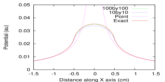
Figure 1: Comparison of potential distribution along X axis

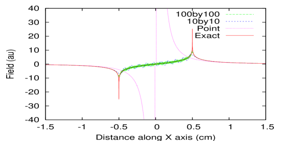
Figure 2: Comparison of $E_{x}$ distribution along X axis

In Table 1, we have presented a comparison of the values of capacitances for a unit square plate and a unit cube as calculated by [Maxwell]-[Mascagni] and our estimations. Although it is difficult to comment regarding which is the best result among the published ones, it is clear from the table that the present solver indeed lead to very accurate results which are well within the acceptable range.

Reference	Method	Plate	Cube
[Maxwell]	Surface Charge	0.3607	-
[Goto]	Refined Surface Charge	$0.3667892\pm 1.1\times 10^{-6}$	$0.6606747\pm 5\times 10^{-7}$
	and Extrapolation
[Read]	Refined Boundary Element	$0.3667874\pm 1\times 10^{-7}$	$0.6606785\pm 6\times 10^{-7}$
	and Extrapolation
[Mansfield]	Numerical Path Integration	0.36684	0.66069
[Mascagni]	Random Walk on the Boundary	-	$0.6606780\pm 2.7\times 10^{-7}$
This work	Boundary Element with	0.3667869	0.6606746
	Exact Expression for Potential

Table 1: Comparison of capacitance values

Finally, in figure 3, the variation of charge density on the top surface of the unit cube has been presented. The sharp increase in charge density near the edges and corners is quite apparent from the figure.

Figure 3: Variation of charge density on the top surface of the cube

4 Conclusions

A fast and accurate BEM solver has been developed using exact expressions for potential and force field due to a uniform source distribution on a flat surface. The expressions have been validated and found to yield very accurate results in the complete physical domain. Of special importance is their ability to reproduce the complicated field structure in the near-field region. The errors incurred in assuming discrete point sources to represent a continuous distribution have been illustrated. Accurate estimates of the capacitance of a unit square plate and that of a unit cube have been made using the new solver. Comparison of the obtained results with very accurate results available in the literature has confirmed the accuracy of the approach and of the solver.