Computation of Electrostatic Field near Three-Dimensional Corners and Edges

N.Majumdar¹ S.Mukhopadhyay¹¹1Saha Institute of Nuclear Physics, 1/AF, Sector 1, Bidhannagar, Kolkata 700064, West Bengal, India, e-mail: nayana.majumdar@saha.ac.in

Abstract

Theoretically, the electric field becomes infinite at corners of two and three dimensions and edges of three dimensions. Conventional finite-element and boundary element methods do not yield satisfactory results at close proximity to these singular locations. In this paper, we describe the application of a fast and accurate BEM solver (which uses exact analytic expressions to compute the effect of source distributions on flat surfaces) to compute the electric field near three-dimensional corners and edges. Results have been obtained for distances as close as 1 $\mu m$ near the corner / edge and good agreement has been observed between the present results and existing analytical solutions.

1 Introduction

Accurate computation of electric field near corners and edges is important in many applications related to science and engineering. While the generic problem is important even in branches like fluid and solid mechanics, the specific electrostatic problem is very important in the modeling and simulation of micro electro-mechanical systems (MEMS), electric probes and antennas, to name a few. While it is true that the ideal corner / edge does not exist in nature, the singularity being smoothed by rounding corners, sharp increase in charge density does occur near these geometries. Since the electric field is proportional to the square of the charge density, it is very important to estimate the charge density and the resulting variation of electric field in their vicinity.

There have been many attempts at solving the above problem using the finite-element (FEM) and the boundary element method (BEM). However, because of the nature of the problem, significant modifications to the basic method needed to be carried out to handle the boundary singularities. On the simpler side, special mesh refinement schemes have been used while on the more sophisticated side, the form of local asymptotic expansions (which may often be found) have been used. Very effective FEM solvers have been developed [Babuska] which calculate singular coefficients by post-processing the numerical solution. These solvers improve the solution by refining the mesh and changing the degree of piecewise polynomials. Similarly, several accurate BEM solvers have been developed [Igarashi], [Elliotis]. For example, in the singular function boundary integral method, the singular coefficients are calculated directly and the solution is approximated by the leading terms of the local asymptotic solution.

In this paper, we present a solution to the corner / edge problem by using a recently developed three-dimensional BEM solver [Mukhopadhyay]. This solver uses exact analytic expressions for computing the influence of charge evenly distributed on discretized flat elements on the boundary. Through the use of these closed-form expressions, the solver avoids one of the most important approximations of the BEM, namely, the assumption that the charge on a boundary element is concentrated at one point (normally the centroid) of the element. As a result, the computed capacitance matrix is very accurate and the solver is able to handle difficult geometries and charge distributions with relative ease. The solver has been used to solve the classic problem of two planes intersecting at various angles. Exact solution to this problem exists [Jackson] and our results have been compared with the exact results. The comparison is very good even as close as 1 $\mu m$ to the corner / edge. Especially important is the fact that the solver produces quite accurate results even for the case of an edge. It has also been possible to reproduce the dependence of the strength of the electric field as a function of the distance from the geometric singularity. All the calculations have been carried out in three dimensions and, here, we also present the variation of the electric field along the corner or edge. It is observed that the electric field retains its mid-plane value for much of the distance along its length, but increases significantly within 20% of the axial ends. It may be noted here that for these calculations, only algebraic mesh refinement near the edge was applied and no other sophisticated techniques such as those mentioned above were applied. This fact made the development of the solver and its application free of mathematical and computational complications. Since corners and edges play an important role in many electro-mechanical structures, the solver can be used to study the electrostatic properties of such geometries.

2 Theory

We have considered the geometry as presented in [Jackson] in which two conducting planes intersect each other at an angle $\beta$ . The planes are assumed to be held at a given potential. A circular cylinder is also included that just encloses the two intersecting plane, has its center at the intersection point and is held at zero potential. The general solution in the polar coordinate system ( $\rho$ , $\phi$ ) for the potential ( $\Phi$ ) close to the origin in this problem has been shown to be

\Phi(\rho,\phi)=V\,+\,{\sum_{m=1}^{\infty}}\,a_{m}\,\rho^{m\pi/\beta}\,sin(m\pi\phi/\beta)

(1)

where the coefficients $a_{m}$ depend on the potential remote from the corner at $\rho=0$ and $V$ represents the boundary condition for $\Phi$ for all $\rho\geq 0$ when $\phi=0$ and $\phi=\beta$ . In the present case where a circular cylinder just encloses the two plates, the problem of finding out $a_{m}$ reduces to a basic fourier series problem with a well known solution

a_{m}\,=\,\frac{4}{m\pi}\,\,\,for\,odd\,m

(2)

It may be noted here that the series in (1) involves positive powers of $\rho^{\pi/\beta}$ , and, thus, close to the origin (i.e., for small $\rho$ ), only the first term in the series will be important. The electric field components ( $E_{\rho},E_{\phi}$ ) are

E_{\rho}(\rho,\phi)=-\frac{\pi}{\beta}{\sum_{m=1}^{\infty}}\,a_{m}\,\rho^{(m\pi/\beta)-1}sin(m\pi\phi/\beta)

(3)

E_{\phi}(\rho,\phi)=-\frac{\pi}{\beta}{\sum_{m=1}^{\infty}}\,a_{m}\,\rho^{(m\pi/\beta)-1}cos(m\pi\phi/\beta)

(4)

Thus, the field components near $\rho=0$ vary with distance as $\rho^{(\pi/\beta)-1}$ and this fact is expected to be reflected in a correct numerical solution as well.

3 Numerical Solution

While the above theoretical solution is a two-dimensional one, we have used the BEM solver to compute a three-dimensional version of the above problem. In order to reproduce the two-dimensional behavior at the mid-plane, we have made the axial length of the system sufficiently long, viz., 10 times the radius of the cylinder. The radius of the cylinder has been fixed at one meter, while the length of the intersecting flat plates has been made a micron shorter than the radius. The length of the plate has been kept smaller than the radius of the cylinder to avoid the absurd situation of having two values of the voltage at the same spatial point. We believe that it has been possible to maintain such a small gap as 1 $\mu m$ between the circular cylinder and the flat plates without facing numerical problems because the BEM solver we have used computes the capacity matrix using analytic expressions which calculate accurate values of potential and electric field at extremely close distances from the singular surfaces [Mukhopadhyay].

The cylinder has been discretized uniformly in the angular and axial directions. The flat plates have also been uniformly discretized in the axial direction. In the radial direction, however, the flat plate elements have been made successively smaller towards the edges using a simple algebraic equation in order to take care of the fact that the surface charge density increases considerably near the edges. The electric field has been computed for various values of $\beta$ ( $1.25\pi,\,1.5\pi,\,1.75\pi\,and\,2\pi$ ), referred to as cases 1, 2, 3 and 4 respectively in the following section.

4 Results

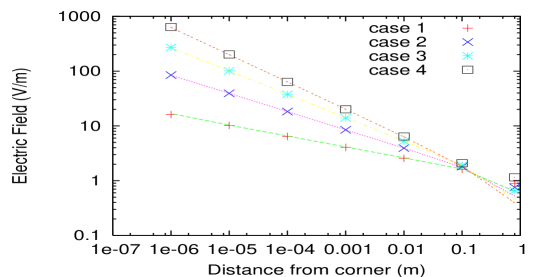
In Figure1, we have presented a comparison of the variation of the electric field as a function of the distance from the edge as found from the analytical solution (3) and the BEM solver. Computations have been carried out upto a distance of 1 $\mu m$ from the edge and to properly represent the sharp increase in field, logarithmic scales have been used. The computed electric field is found to be in remarkable agreement for all values of $\beta$ . There is a small disagreement between the two results only at the point closest to the corner / edge ( $\approx 1.3\%$ ). At present, we are in the process of improving the BEM solver so that this error can be minimized.

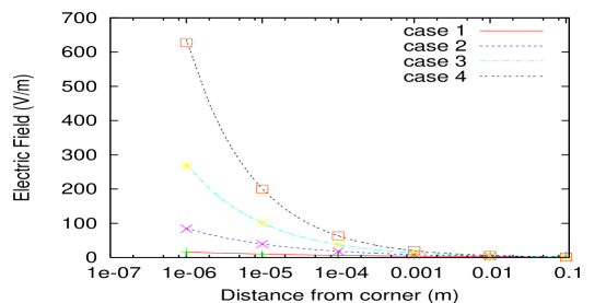
Refer to caption — Figure 1: Comparison of electric field values

Although, the distance dependence of the electric field is expected to match with the theoretical prediction because the computed and the theoretical estimates are found to match closely, in Figure 2, we have plotted curves corresponding to $\rho^{\pi/\beta\,-\,1}$ and compared the computed values as points against the curves. Thus, we can confirm that the computed electric field obeys the $\rho^{(\pi/\beta)\,-\,1}$ relation quite accurately near the corner / edge. Here, to emphasize and visualize the sharpness of the increase of electric field near the singular geometry, only the distance has been drawn using the logscale.

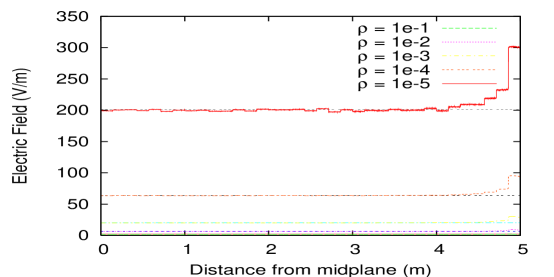
In Figure3, we have presented the variation of the electric field at various distances from the corner / edge along the length of the geometry. While the field is found to increase considerably towards the end, for most of the length ( $\approx 80\%)$ , the two-dimensional value seems to be a good approximation for the real value. However, the deviation (as large as $\approx 50\%$ ) from the analytic solution towards the front and back ends of the geometry should be taken into consideration while designing real-life applications. At close distances near the singular location, oscillation in the electric field value is observed. Initial study indicates that the source of this oscillation is possibly the large size of the boundary elements in the axial direction.

In order to facilitate numerical comparison, we have presented the values of the electric field in the mid-plane as obtained from the exact solution and the BEM solver in Table 1 for the three dimensional edge. We have chosen this case since it is known to be the most difficult among all those considered in this work. It is clear from the table that the present solver does indeed yield very accurate results.

Distance	Exact	Computed	Error (%)
0.1	1.83015317	1.829997	0.0085332
0.01	6.303166063	6.302387	0.012359868
0.001	20.11157327	20.103534	0.039973352
0.0001	63.65561168	63.548305	0.168573794
0.00001	201.31488353	199.998096	0.654093481
0.000001	636.6191357	628.098310	1.33844951

Table 1: Comparison of electric field values

5 Conclusions

A fast and accurate BEM solver has been used to solve the complex problem of finding the electrostatic force field for three dimensional corners and edges. Accurate solutions have been obtained upto distances very close singular geometry. The two dimensional analytic solution has been found to be valid for a large part of the geometry, but near the axial ends, the difference has been found to be significant. The results and the BEM solver is expected to be very useful in solving critical problems associated with the design of MEMS, integrated circuits, electric probes etc. Since these problems are generic in nature, the solver should be important for analysis of problems related to other fields of science and technology.

References

[10]