COMPUTATION OF NEARLY EXACT 3D ELECTROSTATIC FIELD IN GAS IONIZATION DETECTORS

Abstract

The three-dimensional electrostatic field configuration in gas ionization detectors has been simulated using an efficient and precise nearly exact boundary element method (NEBEM) solver set up to solve an integral equation of the first kind. This recently proposed formulation of BEM and the resulting solver use exact analytic integral of Green function to compute the electrostatic potential for charge distribution on flat surfaces satisfying Poisson’s equation. As a result, extremely precise results have been obtained despite the use of relatively coarse discretization leading to successful validation against analytical results available for two-dimensional MWPCs. Significant three dimensional effects have been observed in the electrostatic field configuration and also on the force experienced by the anode wires of MWPCs. In order to illustrate the applicability of the NEBEM solver for detector geometries having multiple dielectrics and degenerate surfaces, it has been validated against available FEM and BEM numerical solutions for similar geometries.

1 INTRODUCTION

Electrostatic forces play a major role in determining gas detector performance. Hence, a thorough understanding of electrostatic properties of gas detectors is of critical importance in the design and operation phases. Computation of electrostatic field is conventionally carried out using one of the following options: analytical approach, finite-element method (FEM), finite-difference approach and boundary element method (BEM). While the first of these possibilities offers the most precise estimation, it is known to be severely restricted in handling of complicated and realistic detector configurations. The FEM is the most popular being capable of producing reasonable results for almost arbitrary geometries [2]. However, for the present task, the FEM is not a suitable candidate because through this method it is possible to calculate potentials only at specific nodal points in the detector volume. For non-nodal points, interpolation becomes a necessity reducing the accuracy significantly. Moreover, numerical differentiation for obtaining field gradients leads to unacceptable electric field values in regions where the gradients change rapidly, for example, near the anode wires of an MWPC. The BEM, despite being capable of yielding nominally exact results while working on a reduced dimensional space(unknowns only on surfaces rather than volumes), suffers from inaccuracies near the boundaries. They also necessitate relatively complicated mathematics.

In this work, we propose the application of a recently formulated Nearly Exact BEM solver (NEBEM) [1] for the computation of electrostatic field in gas detectors. The BEM is a numerical implementation of boundary integral equation (BIE) based on Green’s function method by discretization of the boundary only. For electrostatic problems, the BIE can be expressed as

$$\phi(\vec{r})=\int_{S}{G(\vec{r},{\vec{r}}^{\prime})\rho({\vec{r}}^{\prime})dS^{\prime}}$$ (1)

where $\phi(\vec{r})$ represents the known voltage at $\vec{r}$, $\rho(\vec{r}^{\prime})$ represents the charge density at ${\vec{r}}^{\prime}$, $G(\vec{r},\vec{r}^{\prime})=1/4\pi\epsilon|\vec{r}-\vec{r}^{\prime}|$ and $\epsilon$ is the permittivity of the medium. In order to develop a solver based on this approach, the charge carrying boundaries are segmented on which unknown uniform charge densities ($\rho$) are assumed to be distributed. The unknown $\rho$ and the known $\phi$ are related through the influence matrix $\matrix{A}$

$$\matrix{A}.\rho=\phi$$ (2)

where $A_{ij}$ of $\matrix{A}$ represents the potential at the mid point of segment $i$ due to a unit charge density distribution at the segment $j$. By solving (2), the unknown $\rho$ can be obtained.

Major approximations are made while computing the influences of the singularities which are modeled by a sum of known basis functions with constant unknown coefficients. These approximations ultimately lead to the infamous numerical boundary layer due to which the solution at close proximity of the boundary elements is severely inaccurate.

2 PRESENT APPROACH

In the present approach, we have proposed to use the analytic expressions of potential and force field due to a uniform distribution of singularity on a flat rectangular surface in order to compute highly accurate influence coefficients for the $\matrix{A}$ and for calculations subsequent to the solution of $\rho$. By adopting such an approach, it is possible to improve up on the above-mentioned assumption of singularities concentrated at nodal points and move to uniform charge density distributed on elements. In general, the potential $\phi$ at a point $(X,Y,Z)$ in free space due to uniform source distributed on a rectangular flat surface on the $XZ$ plane and having corners at $(x_{1},0,z_{1})$ and $(x_{2},0,z_{2})$ is known to be a multiple of

$$\phi(X,Y,Z)=\int_{z_{1}}^{z_{2}}\int_{x_{1}}^{x_{2}}\frac{dxdz}{\sqrt{(X-x)^{2}+Y^{2}+(Z-z)^{2}}}$$ (3)

Closed form expressions for the above integration and also for the force vectors have been obtained and used as the foundation expressions of the NEBEM solver described in [1]. It should be noted that these new foundation expressions are valid throughout the physical domain including the close proximity of the singular surfaces. In the present work, we have extended the NEBEM solver to solve the electrostatic problem of gas detectors as follows.

For gas detectors, it is also be useful to model the electrostatics of a wire. For this purpose, we have considered the wires to be thin in comparison to the distance at which the electrostatic properties are being estimated. Under this assumption, the potential $\phi$ at a point $(X,Y,Z)$ due to a wire element along the $Z$ axis of radius $r$ and length $L$ is as follows:

$$\phi=2\pi rlog(\frac{\sqrt{X^{2}+Y^{2}+(Z-h)^{2}}-(Z-h)}{\sqrt{X^{2}+Y^{2}+(Z-h)^{2}}-(Z+h)})$$ (4)

where $r$ is the radius of the wire and $h$ is the half-length of the wire element. Similar expressions for the force field components have also been obtained which are not provided here due to the lack of space. In addition to the expressions given in [1], (4) and the companion force field expressions have been incorporated in the NEBEM solver to compute the electric potential and field in ionization detectors.

3 NUMERICAL IMPLEMENTATION

In this work, we are going to present results related to Iarocci tube, MWPC and RPC. These devices have flat surfaces as their boundaries. The Iarocci tube and the MWPC have anode wires, in addition to the flat conducting surfaces. We have considered Iarocci tubes and MWPCs of various cross-sections ($5mm\times 5mm$ to $16mm\times 16mm$), lengths ($5mm$ to $160mm$) and anode wire diameters ($20\mu m$ to $100\mu m$). The anode wires have been assumed to be held at $1000V$ whereas the other surfaces are assumed to be grounded. The flat surfaces in all these detectors have been segmented in to $21\times 21$ elements. The anode wires have been modeled as cylindrical polygons of 12 sides. Along the axial direction, these cylinders have been segmented in to 21 sub-divisions. These are once again flat surfaces and, thus, have been modeled by the same approach as discussed above. The anode wires have also been represented as thin wires for which (4) and related expressions have performed as foundation expressions. The maximum number of elements with a wire representation for an Iarocci tube has been 1785 while that for a MWPC with five wires have been 1869. Under the assumption of cylindrical polygons, these have increased to 2016 and 3024. These numbers are quite modest and the resulting system can be easily solved on modest desktop computer. Please note that the solver solves a complete three-dimensional problem. We have executed our codes on a Pentium IV machine with 2GB RAM running Fedora Core 3 and it took approximately half an hour of user time to solve the most complicated problem.

4 RESULTS

In this section, we will concentrate mostly on the electric field, rather than the potential, to save space. In Fig.1, we have compared the midplane electric fields computed by the present approach and analytic electric field computed by [2] for a $5mm\times 5mm\times 50mm$ Iarocci tube. It can be seen that the two results match perfectly well. However, when the length of the tube is reduced to $5mm$, the three-dimensionality of the device becomes relevant even at the mid-plane. Thus, in Fig.2 the difference between the two values have become apparent.

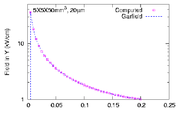
Figure 1: Comparison of electric field at the midplane

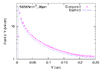
Figure 2: Comparison of electric field at the midplane

In order to illustrate the effect of three-dimensionality, we have presented the relative deviation defined as $Error(\%)=\frac{Garfield-Present}{Garfield}\times 100$ for various Iarocci detectors in Figs.3 and 4. In these figures, results for wires represented as thin wires, as well as cylindrical polygons have also been presented. All the electric fields are at the mid-plane of the 3D detector, the length of which has been varied from 50mm to 5mm. It can be seen that the deviation becomes apparent (close to 1%) as the detector length becomes twice the side of the square detector. When the length is the same as that of the side, the error is as large as 10% near the cathode surfaces. In the latter case, it is more than 2% near the anode wire, which is huge considering the magnitude of the electric field near the anode wire. Fig. 4 illustrates the same point more clearly and, in addition, shows the difference between the two representations of wire. It may be noted that electric field computed by the wire representation seems to be consistently higher than that obtained using the polygon representation.

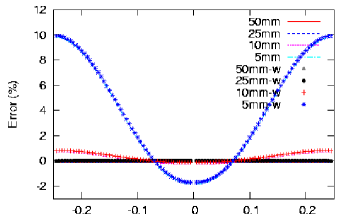
Figure 3: Deviation of electric field at the midplane

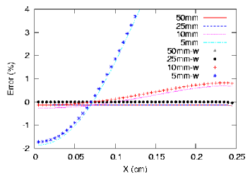
Figure 4: Close up of deviation of electric field at midplane

Next, we present the normal electric field computed along the axial direction of the Iarocci tube in Fig.5. The reference straight line has been provided by using [2] and is the analytic solution for a 2D tube. It can be seen that the 2D value remains valid for almost 85% of the detector along the axial direction. However, in the remaining 15%, 3D effects are quite prominent and hence, non-negligible. There is one more very important point to be noted. Because of the nature of FEM, it almost produces oscillatory results in potential and field (less in the former and more in the latter) near the cathode surface and anode wires. But these are the locations where the results need to be most accurate! By using NEBEM, it has been possible to produce perfectly smooth results without any hint of oscillation. This precision can only be attributed to the exact nature of the foundation expressions of this solver. This remarkable feature of the present solutions should allow more realistic estimation of detector behavior in any situation.

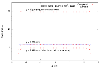
Figure 5: Comparison of normal field along the axial direction

Similar validation and comparisons have been carried out for an MWPC having five anode wires with a wire pitch of $2.5mm$ leading to similar conclusions. There is one feature which is considered to be important mainly for MWPCs, namely, the electrostatic force that acts on the anode wires in an MWPC, especially, its positional variation. In Fig.6, we present the variation of the horizontal force acting on the different anode wires in a five-wire MWPC as we move along the length of the wire. It should be mentioned here that the edge wires in the presented case are of $100\mu m$ diameter, while those inside are of $20\mu m$.

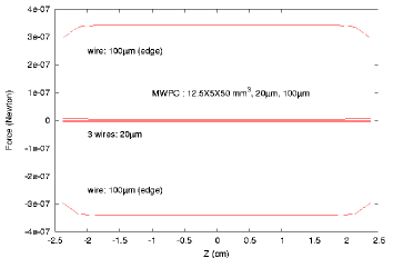
Figure 6: Variation of horizontal force along the axial direction

It is seen that the horizontal force becomes quite considerable as we move towards the edge of the detector despite the use of larger diameter wire as guard wires.

In the following Fig.7, we have presented the normal electric field contour at the mid-plane of the detector. The sharp increase in the magnitude of this field is quite evident near the wire locations.

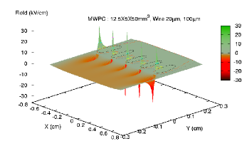
Figure 7: Surface and contour plots of the normal electric field

Several detector configurations in current use such as MSGC, RPC, GEM have multiple dielectric configuration. They also have extremely thin charged surfaces such as the graphite coatings of RPCs. Such surfaces may necessitate treatment of degenerate surfaces. As a result, in the following, we have tried to validate the NEBEM solver by computing the electrostatic properties of such configurations and comparing them with FEM and Dual BEM (DBEM) results given in [3] where the problem geometry is discussed in detail. In the following Tables 1, 2 and 3, we present the comparison among the potentials as computed by the above three approaches. It is obvious from these results that the agreement is excellent despite the use of only $11\times 11$ discretization of the surfaces. Please note that in the tables $R$ denotes the ratio between the permittivity of two slabs placed on top of another (upper/lower) and the locations are expressed in microns.

Table 1: Comparison for R = 10

Location	FEM	DBEM	NEBEM
18.0,3.0	0.1723103	0.17302	0.1740844
4.0,9.0	0.2809692	0.27448	0.2807477
25.0,16.0	0.6000305	0.59607	0.5991884
5.0,17.0	0.679071	0.67492	0.6785017

Table 2: Comparison for R = 0.1

Location	FEM	DBEM	NEBEM
18.0,3.0	0.01741943	0.017302	0.0171752
4.0,9.0	0.0281006	0.027448	0.0286358
25.0,16.0	0.4883313	0.480640	0.4828946
5.0,17.0	0.5929200	0.589690	0.5926387

Table 3: Comparison for R = 10

Location	FEM	DBEM	NEBEM
24.0,16.5	0.514489	0.52181	0.5247903
6.5,12.0	0.230147	0.23801	0.2398346
22.5,6.0	0.3638855	0.34638	0.3451232
4.0,3.5	0.1108643	0.10623	0.1058357

Finally, in Fig.8, we have presented the electric field configuration of an RPC computed using NEBEM. The RPC is assumed to have 2mm gas gap enclosed by two 2mm glass. On the two outer surfaces of the glass, graphite coating has been applied. The upper graphite coating has been raised to 8kV, while the lower one is grounded. The RPC is 10mm wide, enclosed on the left and right sides by glass and has a similar spacer in the middle. The variation of the electric field along the vertical direction (Y) on the midplane at various X locations have been presented. It can be seen that the normal electric field rises up to around 40kV/cm in the gas gap of the RPC.

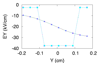
Figure 8: Electric field in an RPC

5 CONCLUSION

Thus, it may be concluded that

Precise computation of three-dimensional surface charge density, potential and electrostatic field has been carried out for gas ionization detectors using the Nearly Exact BEM (NEBEM) solver.

The NEBEM yields precise results for a very wide range of realistic electrostatic configurations including multiple dielectric systems.

As future plans we have the following aspects

Optimization of the NEBEM solver.

Multiphysics nature of NEBEM needs to be explored. After all, the foundation expressions represent new solutions to the Poisson equation which is one of the most important equations in physics!

Applications to other areas will be explored

6 ACKNOWLEDGEMENTS

We would like to acknowledge the help and encouragement of Prof. Bikash Sinha, Director, SINP and Prof. Sudeb Bhattacharya, Head, Nuclear and Atomic Physics, SINP throughout the period of this work.

References

- [1] S.Mukhopadhyay, N.Majumdar, ”Development of a BEM Solver using Exact Expressions for Computing the Influence of Singularity Distributions”, ICCES05, Chennai, December 2005.
- [2] http://garfield.web.cern.ch/garfield
- [3] S-W Chyuan, Y-S Liao, J-T Chen, ”An efficient technique for solving the arbitrarily multilayered electrostatic problems with singularity arising from a degenerate boundary”, Semicond. Sci. Technol. 19, R47(2004).