“Universal” Distribution of Inter-Earthquake Times Explained

Abstract

We propose a simple theory for the “universal” scaling law previously reported for the distributions of waiting times between earthquakes. It is based on a largely used benchmark model of seismicity, which just assumes no difference in the physics of foreshocks, mainshocks and aftershocks. Our theoretical calculations provide good fits to the data and show that universality is only approximate. We conclude that the distributions of inter-event times do not reveal more information than what is already known from the Gutenberg-Richter and the Omori power laws. Our results reinforces the view that triggering of earthquakes by other earthquakes is a key physical mechanism to understand seismicity.

Understanding the space-time-magnitude organization of earthquakes remains one of the major unsolved problem in the physics of the Earth. Earthquakes are characterized by a wealth of power laws, among them, (i) the Gutenberg-Richter distribution $\sim 1/E^{1+\beta}$ (with $\beta\approx 2/3$) of earthquake energies $E$ KKK ; (ii) the Omori law $\sim 1/t^{p}$ (with $p\approx 1$ for large earthquakes) of the rate of aftershocks as a function of time $t$ since a mainshock utsu ; (iii) the productivity law $\sim E^{a}$ (with $a\lesssim 2/3$) giving the number of earthquakes triggered by an event of energy $E$ H ; (iv) the power law distribution $\sim 1/L^{2}$ of fault lengths $L$ Davy ; (v) the fractal (and even probably multifractal MultiSO ) structure of fault networks davy2 and of the set of earthquake epicenters KK . The quest to squeeze novel information from the observed properties of seismicity with ever new ways of looking at the data goes unabated in the hope of better understanding the physics of the complex solid Earth system. In this vein, from an analysis of the probability density functions (PDF) of waiting times between earthquakes in a hierarchy of spatial domain sizes and magnitudes in Southern California, Bak et al. discussed in 2002 a unified scaling law combining the Gutenberg-Richter law, the Omori law and the fractal distribution law in a single framework Baketal (see also ref. Kosso for a similar earlier study). This global approach was later refined and extended by the analysis of many different regions of the world by Corral, who proposed the existence of a universal scaling law for the PDF $H(\tau)$ of recurrence times (or inter-event times) $\tau$ between earthquakes in a given region $\mathcal{S}$ Corral1 ; Corral2 :

$$H(\tau)\simeq\lambda f(\lambda\tau)~{}.$$ (1)

The remarkable finding is that the function $f(x)$, which exhibit different power law regimes with cross-overs, is found almost the same for many different seismic regions, suggesting universality. The specificity of a given region seems to be completely captured solely by the average rate $\lambda$ of observable events in that region, which fixes the only relevant characteristic time $1/\lambda$.

The common interpretation is that the scaling law (1) reveals a complex spatio-temporal organization of seismicity, which can be viewed as an intermittent flow of energy released within a self-organized (critical?) system SS89Baktang , for which concepts and tools from the theory of critical phenomena can be applied CorralRG . Beyond these general considerations, there is no theoretical understanding for (1). Under very weak and general conditions, Molchan proved mathematically that the only possible form for $f(x)$, if universality holds, is the exponential function Molchan , in strong disagreement with observations. Recently, from a re-analysis of the seismicity of Southern California, Molchan and Kronrod MolchanKontrov have shown that the unified scaling law (1) is incompatible with multifractality which seems to offer a better description of the data.

Here, our goal is to provide a simple theory, which clarifies the status of (1), based on a largely studied benchmark model of seismicity, called the Epidemic-Type Aftershock Sequence (ETAS) model of triggered seismicity Ogata and whose main statistical properties are reviewed in HS02 . The ETAS model treats all earthquakes on the same footing and there is no distinction between foreshocks, mainshocks and aftershocks: each earthquake is assumed capable of triggering other earthquakes according to the three basic laws (i-iii) mentioned above. The ETAS model assumes that earthquake magnitudes are statistically independent and drawn from the Gutenberg-Richter distribution $Q(m)$. Expressed in earthquake magnitudes $m\propto(2/3)\ln_{10}E$, the probability $Q(m)$ for events magnitudes $m_{i}$ to exceed a given value $m$ is $Q(m)=10^{-b(m-m_{0})}$, where $b\simeq 1$ and $m_{0}$ is the smallest magnitude of triggering events. We also parametrize the (bare) Omori law for the rate of triggered events of first-generation from a given earthquake as $\Phi(t)=\theta c^{\theta}/(c+t)^{1+\theta}$, with $\theta\gtrsim 0$. $\Phi(t)$ can be interpreted as the PDF of random times of independently occurring first-generation aftershocks triggered by some mainshock which occurred at the origin of time $t=0$. Several authors have shown that the ETAS model provides a good description of many of the regularities of seismicity (see for instance Ref. SS_EPJB and references therein).

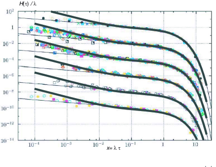
Figure 1: Fig.1 taken from Corral’s Ref.Corral2 plotting the scaled (according to (1) probability density functions (PDF) of the recurrence times $\tau$ between successive earthquakes in various regions of the world, scaled by their corresponding seismicity rates $\lambda$. Top to bottom: the NEIC worldwide catalog for regions with $L\geq 180$ degrees, 1973-2002; NEIC with $L\leq 90$ degrees, (same period of time); Southern California, 1984-2001, 1988-1991, and 1995-1998; Northern California, 1998-2002; Japan, 1995-1998, and New Zealand, 1996-2001; (bottom), Spain, 1993-1997, New Madrid, 1975-2002, and Great Britain, 1991-2001. The PDFs have been translated for clarity. The thin continuous lines are Corral’s fits (12) while the thick continuous lines are our prediction (11) based on ETAS model with the parameters $\theta=0.03,n=0.9,a=0.76$ and $\rho=1$.

Our main result is the theoretical prediction (11) below, which is used to fit Corral’s data in Fig. 1, with remarkably good agreement. According to Occam’s razor, this suggests that the previously mentioned results on universal scaling laws of inter-event times do not reveal more information that what is already captured by the well-known laws (i-iii) of seismicity (Gutenberg-Richter, Omori, essentially), together with the assumption that all earthquakes are similar (no distinction between foreshocks, mainshocks and aftershocks HS03 ), which is the key ingredient of the ETAS model. Our theory is able to account quantitatively for the empirical power laws found by Corral, showing that they result from subtle cross-overs rather than being genuine asymptotic scaling laws. We also show that universality does not strictly hold.

Our strategy to obtain these results is to first calculate the PDF of the number of events in finite space-time windows SS_EPJB , using the technology of generating probability functions (GPF), which is particularly suitable to deal with the ETAS as it is a conditional branching process. We then determine the probability for the absence of earthquakes in a given time window from which, using the theory of point processes, is determined the PDF of inter-event times. Our analysis is based the previous calculations of Ref. SS_EPJB , which showed that, for large areas ($L\sim$ tens of kilometers or more), one may neglect the impact of aftershocks triggered by events that occurred outside the considered space window, while only considering the events within the space domain which are triggered by sources also within the domain.

Generating probability functions of the statistics of event numbers. Consider the statistics of the number $R(t,\tau)$ of events within a time window $[t,t+\tau]$. It is efficiently described by the method of GPF, defined by $\Theta_{s}(z,\tau)=\langle z^{R(t,\tau)}\rangle$ where the brackets $\langle.\rangle$ denote a statistical average over all possible realizations weighted by their corresponding probabilities. We consider a statistically stationary process, so that $\Theta_{s}(z,\tau)$ does not depend on the current time $t$ but only on the window duration $\tau$. For the ETAS model, statistical stationarity is ensured by the two conditions that (i) the branching ratio $n$ (or average number of earthquakes/aftershocks of first-generation per earthquake) be less than $1$ and (ii) the average rate $\omega$ of the Poissonian distribution of spontaneous events be non-zero. The GPF $\Theta_{s}(z,\tau)$ can then be obtained as SS_EPJB

$$\Theta_{s}(z,\tau)=\exp\left(-\omega\int^{\infty}_{0}[1-\Theta(z,t,\tau)]\,dt-\omega\int^{\tau}_{0}[1-z\Theta(z,t)]\,dt\right)~{},$$ (2)

where $\Theta(z,t,\tau)$ is the GPF of the number of aftershocks triggered inside the window $[t,t+\tau]$ ($t>0$) by a single isolated mainshock which occurred at time $0$ and $\Theta(z,\tau)=\Theta(z,t=0,\tau)$. The first (resp. second) term in the exponential in (2) describes the contribution of aftershocks triggered by spontaneous events occurring before (resp. within) the window $[t,t+\tau]$.

Ref. SS_EPJB previously showed that $\Theta(z,t,\tau)$ is given by

$$\Theta(z,t,\tau)=G[1-\Psi(z,t,\tau)]~{},$$ (3)

where $G(z)$ is the GPF of the number of first-generation aftershocks triggered by some mainshock, and the auxiliary function $\Psi(z,t,\tau)$ satisfies to

$$\Psi(z,t,\tau)=\left[1-\Theta(z,t,\tau)\right]\otimes\Phi(t)+\left[1-z\Theta(z,\tau)\right]\otimes\Phi(t+\tau)~{}.$$ (4)

The symbol $\otimes$ denotes the convolution operator. Integrating (4) with respect to $t$ yields $\int_{0}^{\infty}\Psi(z,t,\tau)\,dt=\int^{\infty}_{0}[1-\Theta(z,t,\tau)]\,dt+\left[1-z\Theta(z,\tau)\right]\otimes a(\tau)$, so that expression (2) becomes

$$\Theta_{s}(z,\tau)=\exp\left[-\omega\int_{0}^{\infty}\Psi(z,t,\tau)\,dt-\omega\left[1-z\Theta(z,\tau)\right]\otimes b(\tau)\right]\,,$$ (5)

where $b(t)=\int_{0}^{t}\Phi(t^{\prime})\,dt^{\prime}$ and $a(t)=1-b(t)={c^{\theta}\over(c+t)^{\theta}}$.

Probability of abscence of events. For our purpose, the probability $P_{s}(\tau)$ that there are no earthquakes in a given time window of duration $\tau$ provides an intuitive and powerful approach. It is given by

$$P_{0}(\tau)\equiv\Theta_{s}(z=0,\tau)=\exp\left[-\omega\int_{0}^{\infty}\Psi(t,\tau)\,dt-\omega\tau+\omega A(\tau)\right]~{},$$ (6)

where $\Psi(t,\tau)=\Psi(z=0,t,\tau)$ and $A(\tau)=\int_{0}^{\tau}a(t)dt\simeq{c\over 1-\theta}\left(\tau/c\right)^{1-\theta}$, for $\tau\gg c)$.

To make progress in solving (3,4,5), let us expand $G(z)$ in powers of $z$:

$$G(z)=1-n+nz+\beta(1-z)^{\gamma}+...~{},$$ (7)

where $\gamma=b/\alpha$ (where $\alpha=(3/2)a<1$ is the productivity exponent when using magnitudes) and $\beta=n\Gamma(2-\gamma)(\gamma-1)^{\gamma-1}/\gamma^{\gamma}$. While we can calculate the looked-for distribution of recurrence times using the shown expansion up to order $(1-z)^{\gamma}$, it turns out that truncating (7) at the linear order is sufficient to explain quantitatively Corral’s results, as we show below. Using $G(z)=1-n+nz$ has the physical meaning that each earthquake is supposed to generate at most one first-generation event (which does not prevent it from having many aftershocks when summing over all generations). Indeed, interpreted in probabilistic term, $G(z)=1-n+nz$ says that any earthquake has the probability $1-n$ to give no offspring and the probability $n$ to give one aftershock (of first-generation). This linear approximation is bound to fail for small recurrence times associated with the large productivity of big earthquakes and, indeed, we observe some deviations for the shorter recurrence times below several minutes as discussed below. The linear approximation is not intended to describe the statistics of very small recurrence times within clusters of events triggered by large mainshocks, but is approprioate for “quiet” periods of seismic activity. The linear approximation is expected and actually seen to work remarkably well for large recurrence times of hours, days, weeks…

The linear approximation bypasses much of the complexity of the nonlinear integral equations (3,4) to obtain $\int_{0}^{\infty}\Psi(t,\tau)dt={A(\tau)\over 1-n}$. Expression (6) becomes (for $\tau\gg c$)

$$P_{s}(\tau)=\exp\left[-(1-n)x-{na\rho^{\theta}\over 1-\theta}~{}x^{1-\theta}\right]~{},$$ (8)

where

$$x=\lambda\tau~{},~{}~{}~{}a=(\lambda_{0}c)^{\theta}~{},~{}~{}~{}\rho=\lambda/\lambda_{0}=Q(m)\left({L\over L_{0}}\right)^{d}~{}.$$ (9)

The average seismicity rate $\lambda$ is given by $\lambda={\omega\over 1-n}$, which renormalizes the average rate $\omega$ of spontaneous sources by taking into account earthquakes of all generations triggered by a given source: $\lambda=\omega+n\omega+n^{2}\omega+...$. Due to the assumed statistical independence between event magnitudes, the proportion between spontaneous observable events and their observable aftershocks does not depend on the magnitude threshold and the above expression for the average seismic rate holds also for observable events at different magnitude thresholds of completeness. Finally, $\lambda_{0}$ is the average seismic rate within a spatial domain $\mathcal{S}_{0}$ of reference with linear size $L_{0}$, and $\rho$ takes into account the dependence on the magnitude threshold $m$ for observable events and on the scale $L$ of the spatial domain $\mathcal{S}$ used in the analysis. The first term $(1-n)x$ in the exponential of (8) describes the exponential decreasing probability of having no events as $\tau$ increases due to the spontaneous occurrence of sources. The other term proportional to $x^{1-\theta}$ takes into acount the influence through Omori’s law of earthquakes that happened before the time window.

Statistics of recurrence times. Consider a sequence of times $\{t_{i}\}$ of observable earthquakes, occurring inside a given seismic area $\mathcal{S}$. The inter-event times are by definition $\tau_{i}=t_{i}-t_{i-1}$. The whole justification for the calculation of $P_{s}(\tau)$ lies in the well-known fact in the theory of point processes ptp that the PDF $H(\tau)$ of recurrence times $\tau_{i}$ is given by the exact relation

$$H(\tau)={1\over\lambda}{d^{2}P_{s}(\tau)\over d\tau^{2}}~{}.$$ (10)

Substituting (8) in this expression yields our main theoretical prediction for the PDF of recurrence times, which is found to take the form (1) with

$$\begin{array}[]{c}f(x)=\left(an\theta\rho^{\theta}x^{-1-\theta}+\left[1-n+na\rho^{\theta}x^{-\theta}\right]^{2}\right)\\[5.69054pt] \displaystyle\exp\left(-(1-n)x-{na\rho^{\theta}\over 1-\theta}~{}x^{1-\theta}\right)~{}.\end{array}$$ (11)

While our theoretical derivation justifies the scaling relation (1) observed empirically Corral1 ; Corral2 , the scaling function $f(x)$ given by (11) is predicted to depend on the criticality parameter $n$, the Omori law exponent $\theta$, the detection threshold magnitude $m$ and the size $L$ of the spatial domain $\mathcal{S}$ under study. While $\theta$ might perhaps be argued to be universal, this is less clear for $n$ which could depend on the regional tectonic context. The situation seems much worse for universality with respect to the two other parameters $m$ and $L$ which are catalog specific. It thus seems that our prediction can not agree with the finding that $f(x)$ is reasonably universal over different regions of the world as well as for worldwide catalogs Corral1 ; Corral2 .

It turns out that the dependence on the idiosynchratic catalog-dependent parameters $m$ and $L$ is basically irrelevant as long as $\theta$ is small and $n$ in the range $0.7-1$ previously found to be consistent with several other statistical properties of seismicity SSlifetime ; SS_EPJB . Note that the condition that $\theta$ be small is fully compatible with many empirical studies in the literature for the Omori law reporting an observable (renormalized) Omori law decay $\sim 1/t^{0.9-1}$ corresponding to $\theta=0-0.1$ HS02 . Fig. 2 shows the changes of $f(x)$ when varying the magnitude threshold from $0$ to $3$. These changes of $f(x)$ seem to be within the inherent statistical uncertainties observed in empirical studies Corral1 ; Corral2 . The technical origin of the robustness lies in the fact that, for $\theta=0.03$ say, changing $m-m_{0}$ from $0$ to $6$ amounts to changing $\rho$ from $1$ ($m=m_{0}$) to $\rho=10^{-6}$ ($m=m_{0}+6$) which changes $\rho^{\theta}$ from 1 to only $\rho^{\theta}\simeq 0.66$. We conclude that our theory provides an explanation for both the scaling ansatz (1) and its apparent universal scaling function.

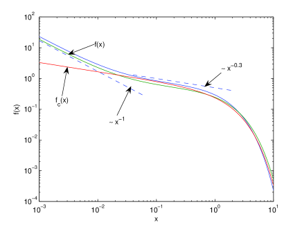
Figure 2: Scaling function $f(x)$ defined in (11) for $n=0.8$, $\theta=0.03$, $a=0.76$ and for two values of $m-m_{0}=0,3$ corresponding to a thousand-fold variation of $\rho=1;10^{-3}$. In these synthetic examples, we assume that the spatial domain $\mathcal{S}_{0}$ corresponds to an average seismicity rate $\lambda_{0}\simeq 1$ per day, that the characteristic time scale of the Omori law is $c\simeq 10$ sec., so that $\lambda_{c}\simeq 10^{-4}$. Then, for $\theta\simeq 0.03$, we have $a\simeq 0.76$. The obtained function $f(x)$ is compared with Corral’s empirical fitting function $f_{c}(x)$ defined in (12) with $g=0.7$, $\delta=1.05$, $d=1.7$ and $C=0.78$. The dashed lines are the power laws $\sim x^{-0.3}$ and $x^{-1}$.

We can squeeze more out of (11) to rationalize the empirical power laws reported by Corral. In particular, Corral proposed the following empirical form for $f(x)$ which, in our notations, reads

$$f_{c}(x)={C\delta\over d\Gamma(\gamma/\delta)}\left({x\over d}\right)^{g-1}e^{-(x/d)^{\delta}}~{},$$ (12)

where $g=0.67\pm 0.05,\delta=1.05\pm 0.05,d=1.64\pm 0.15$, and $C$ ensures normalization Corral1 ; Corral2 . Fig.2 shows indeed that expression (12) with Corral’s reported parameter values for $g,\delta$ and $d$ fits (11) remarkably well quantitatively. While the intermediate asymptotics $f(x)\sim x^{\gamma-1}\simeq x^{-0.3}$ proposed by Corral is absent from our theoretical expression (11), it can actually be seen as a long cross-over between the power and exponential factors in (11), as shown by one of the dashed lines in Fig.2.

Interestingly, expressions (11) and (12) depart from each other for $x\lesssim 0.01$. Our theoretical distribution $f(x)$ has the power law asymptotic $f(x)\sim x^{-1}$, which is a direct consequence of Omori’s law described explicitly by the first power law factor in front of the exponential in (11). It is absent from expression (12). However, its presence is clear in real data as shown in Fig. 1 extracted from Corral2 on which we have superimposed our theoretical prediction (11). Note that expression (11) exhibits a slight departure from the data for small $x$’s (defined in (9)), which can be attributed to the linearization of (7), which amounts to neglecting the renormalization of the Omori law by the cascade of triggered aftershocks HS02 . Taking into account this renormalization effect by the higher-order terms in the expansion (7) improves the fit to the data shown in Fig. 1. Our detailed study shows that comparing (11) with data provides constraints on the parameter $n$: the data definitely excludes small values of $n$ and seems best compatible with $n=0.7-1$, in agreement with previous constraints SS_EPJB suggesting that earthquake triggering is a dominant process.

References

- (1) L. Knopoff, Y.Y. Kagan and R. Knopoff, Bull. Seism. Soc. Am. 72, 1663-1676 (1982).
- (2) T. Utsu, Y. Ogata and S. Matsu’ura, J. Phys. Earth 43, 1-33 (1995).
- (3) A. Helmstetter, Y. Kagan and D. Jackson, J. Geophys. Res., 110, B05S08, 10.1029/2004JB003286 (2005).
- (4) Sornette, D. and P. Davy, Geophys. Res.Lett. 18, 1079 (1991).
- (5) D. Sornette and G. Ouillon, Phys. Rev. Lett. 94, 038501 (2005).
- (6) Davy, P., A. Sornette and D. Sornette, Nature 348, 56-58 (1990).
- (7) Kagan, Y.Y. and L. Knopoff, Geophys. J. Roy. Astr. Soc., 62, 303-320 (1980).
- (8) P. Bak et al., Phys. Rev. Lett. 88, 178501 (2002).
- (9) V.G. Kossobokov and S.A. Mazhkenov, Spatial characteristics of similarity for earthquake sequences: Fractality of seismicity, Lecture Notes of the Workshop on Global Geophysical Informatics with Applications to Research in Earthquake Prediction and Reduction of Seismic Risk (15 Nov.-16 Dec., 1988), ICTP, 1988, Trieste, 15 p. (1988).
- (10) A. Corral, Phys. Rev. E 68, 035102 (2003).
- (11) A. Corral, Physica A 340, 590 (2004).
- (12) A. Sornette and D. Sornette, Europhys.Lett. 9, 197-292 (1989); P. Bak and C. Tang, J. Geophys. Res. 94, 15,635 (1989).
- (13) A. Corral, Phys. Rev. Lett. 95 028501 (2005).
- (14) G.M. Molchan, Pure appl. geophys., 162, 1135-1150 (2005).
- (15) G. Molchan and T. Kronrod, Seismic Interevent Time: A Spatial Scaling and Multifractality, physics/0512264 (2005).
- (16) Y. Ogata, J. Am. Stat. Assoc. 83, 9 (1988); Y.Y. Kagan and L. Knopoff, J. Geophys. Res. 86, 2853 (1981).
- (17) A. Helmstetter and D. Sornette, J. Geophys. Res. 107, B10, 2237 (2002).
- (18) A. Saichev and D. Sornette, Eur. J. Phys. B 49, 377 (2006).
- (19) Helmstetter, A. and D. Sornette, J. Geophys. Res. 108, 10.1029, 2457, 2003.
- (20) D.J. Daley, D. Vere-Jones, An Introduction to the Theory of the Point Processes. New York, Berlin: Springer-Verlag, 1988, 702 pp.
- (21) A. Saichev and D. Sornette Phys. Rev. E 70, 046123 (2004); Phys. Rev. E 71, 056127 (2005).