Multi-asset minority games

Abstract

We study analytically and numerically Minority Games in which agents may invest in different assets (or markets), considering both the canonical and the grand-canonical versions. We find that the likelihood of agents trading in a given asset depends on the relative amount of information available in that market. More specifically, in the canonical game players play preferentially in the stock with less information. The same holds in the grand canonical game when agents have positive incentives to trade, whereas when agents payoff are solely related to their speculative ability they display a larger propensity to invest in the information-rich asset. Furthermore, in this model one finds a globally predictable phase with broken ergodicity.

I Introduction

The study of systems of heterogeneous adaptive agents through Minority Games (MGs) ElFarol ; CZ has attracted much interest from statistical physicists. Despite the simplicity of the interactions between agents, these models generate rich static and dynamical structures which can often be well understood at the mathematical level through the use of spin-glass techniques book ; cool . While the MG has found applications in different types of problems (see for example traffic ), it was originally designed to address the issue of how the microscopic behavior of traders – speculators in particular – may give rise to the anomalous global fluctuation phenomena observed empirically in financial markets. In this respect the most successful version of the MG has perhaps been the grand-canonical MG Johnson ; GCMG , in which traders may abstain from investing, so that the traded volume fluctuates in time.

The core of MGs is the assumption that traders react to the receipt of an information pattern (be it exogenous or endogenous) by taking a simple trading decision such as buying or selling. The key control parameter is the ratio between the number of traders and the ‘complexity’ of the information space, measured by the number of possible patterns. In general, when this ratio exceeds a certain threshold MGs undergo a phase transition to a macroscopically efficient state where it is not possible to predict statistically whether a certain decision will be fruitful or not based on the received information alone.

Real markets are typically formed by different assets and are characterized by non trivial correlations Mantegna ; Potters ; Kertesz . These correlations arise from the underlying behavior of the economics (the fundamentals) but they are also “dressed” by the effect of financial trading. In this paper, we will use the Minority Game in order to investigate how speculative trading affects the different assets in a market. Versions of MG where agents are engaged in different contexts have already been introduced and studied Rodgers ; Chau . More precisely, we shall investigate how speculative trading contributes to financial correlations, and how speculators distribute their trading volume depending on the information content of the different asset markets.

Our first result is that speculative trading does not contribute in a sensible manner to financial correlations, and if it does, it likely contributes a negative correlation. The reason is that, within the schematic picture of the MG, speculators are uniquely driven by profit considerations and totally disregard risk. The same cannot be said for strategies on lower frequencies (buy and hold) where risk minimization of the portfolio becomes important.

Our second main conclusion is that, when there are positive incentives to trade, speculators invest preferentially on the asset with the smallest information content. This apparently paradoxical conclusion is reverted when speculators have no incentive to trade, other than making a profit. This is due to the fact that speculators, when they are forced to trade also contribute to information asymmetries.

Finally, with respect to the usual classification in phases of the MG, we find a considerably richer phase diagram where different components of the market may be in different phases. These conclusions are derived for the case of a market composed of two assets, which allows for a simpler treatment and provides a more transparent picture. Their validity can be extended in straightforward ways to the case of markets with a generic number of assets.

The paper is articulated in three parts. Section II is dedicated to the study of a canonical MG where agents can choose on which of two assets to invest. In Section III we discuss the grand-canonical version of this model, where agents are also allowed to refrain from investing. Finally, we formulate our conclusions in Sec. IV. The mathematical analysis of the models we consider is a generalization of calculations abundantly discussed in the literature (see book ; cool for recent reviews). We therefore won’t go into the details, limiting ourselves to stressing the main differences with the standard cases.

II Canonical Minority Game with two assets

We consider the case of a market with two assets $\gamma\in\{-1,1\}$ and $N$ agents. At each time step $t$, agents receive two information patterns $\mu_{\gamma}\in\{1,\ldots,P_{\gamma}\}$, chosen at random and independently with uniform probability. It is assumed that $P_{\gamma}$ scales linearly with $N$, and their ratio is denoted by $\alpha_{\gamma}=P_{\gamma}/N$. Every agent $i$ disposes of two “strategies” $\bm{a}_{i\gamma}=\{a_{i\gamma}^{\mu_{\gamma}}\}$ (one for each asset), that prescribe a binary action $a_{i\gamma}^{\mu_{\gamma}}\in\{-1,1\}$ (buy/sell) for each possible information pattern. Each component $a_{i\gamma}^{\mu_{\gamma}}$ is assumed to be selected randomly and independently with uniform probability and is kept fixed throughout the game. Traders keep tracks of their performance in the different markets through a score function $U_{i\gamma}(t)$ which is updated with the following rule:

$$U_{i\gamma}(t+1)=U_{i\gamma}(t)-a^{\mu_{\gamma}(t)}_{i\gamma}A_{\gamma}(t)$$ (1)

where

$$A_{\gamma}(t)=\sum_{j=1}^{N}a^{\mu_{\gamma}(t)}_{j\gamma}\delta_{s_{j}(t),\gamma}$$ (2)

represents the ‘excess demand’ or the total bid on market $\gamma$ (the factor $1/\sqrt{N}$ appears here for mathematical convenience) and is usually taken as a proxy of (log) returns, i.e. $\log p_{\gamma}(t+1)=\log p_{\gamma}(t)+\lambda A_{\gamma}(t)$. The Ising variable

$$s_{i}(t)=\hbox{sign}\,\left[U_{i,+1}(t)-U_{i,-1}(t)\right]$$ (3)

indicates the asset in which player $i$ invests at time $t$, which is simply the one with the largest cumulated score. It is the minus sign on the right-hand side of (1) that enforces the minority-wins rule in both markets: Agents will invest in that market where their strategy provides a larger payoff $-a_{i\gamma}^{\mu_{\gamma}(t)}A_{\gamma}(t)$ (or a smaller loss).

It is possible to characterize the asymptotic behaviour of the multi-agent system (1) with a few macroscopic observables, such as the predictability $H$ and the volatility $\sigma^{2}$, defined respectively as H

$$H=\sum_{\gamma\in\{-1,1\}}\frac{1}{NP_{\gamma}}\sum_{\mu_{\gamma}=1}^{P_{\gamma}}\left\langle{A_{\gamma}|\mu_{\gamma}}\right\rangle^{2}=H_{+}+H_{-}$$ (4)

$$\sigma^{2}=\frac{1}{N}\sum_{\gamma}\left\langle{A_{\gamma}^{2}}\right\rangle=\sigma^{2}_{+}+\sigma^{2}_{-}$$ (5)

with $\left\langle{\cdot}\right\rangle$ and $\left\langle{\cdot|\mu_{\gamma}}\right\rangle$ denoting time averages in the steady state, the latter conditioned on the occurrence of the information pattern $\mu_{\gamma}$. Besides these, in the present case, it is also important to study the relative propensity of traders to invest in a given market, namely

$$m=\frac{1}{N}\sum_{i=1}^{N}\left\langle{s_{i}}\right\rangle$$ (6)

A positive (resp. negative) $m$ indicates that agents invest preferentially in asset $+1$ (resp. $-1$).

It is clear, already at this stage, that if no a priori correlation is postulated between the news arrival processes on the two assets $\mu_{\pm}(t)$ or between the strategies adopted by agents in the two markets, no correlation is created by agents. Indeed

$$\left\langle{A_{+}A_{-}}\right\rangle=\frac{1}{N}\sum_{i,j}\left\langle a_{i,+}^{\mu_{+}}a_{i,-}^{\mu_{-}}\frac{1+s_{i}}{2}\frac{1-s_{j}}{2}\right\rangle$$ (7)

and we know MC01 that dynamical variables $U_{i\gamma}(t)$ evolve on timescales much longer (of order $P_{\gamma}$) than that over which $\mu_{\gamma}$ changes. Hence we can safely assume that the distribution of $s_{i}$ in Eq. (7) is independent of $\mu_{\pm}$, which allows to factor the average $\langle a_{i,+}^{\mu_{+}}a_{i,-}^{\mu_{-}}\rangle=\langle a_{i,+}^{\mu_{+}}\rangle\langle a_{i,-}^{\mu_{-}}\rangle$ over the independent information arrival processes $\mu_{\pm}(t)$. Given that $\langle a_{i,\pm}^{\mu_{\pm}}\approx 0$ we conclude that $\left\langle{A_{+}A_{-}}\right\rangle\approx 0$ also. The reason for this is that traders behavior is aimed at detecting excess returns in the market with no consideration about the correlation among assets. The quantities defined above can be obtained both numerically and analytically (in the limit $N\to\infty$) as functions of $\alpha_{+}$ and $\alpha_{-}$. The phase structure of the model is displayed in Fig. 1.

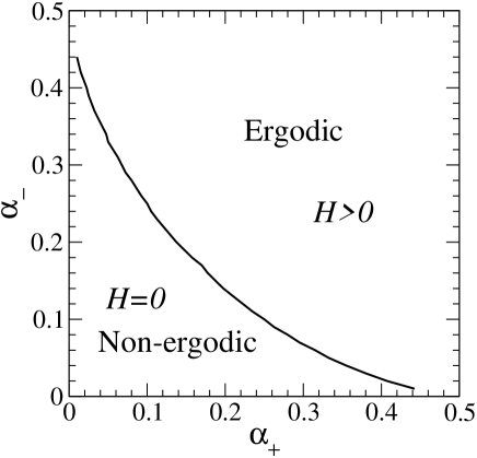
Figure 1: Analytical phase diagram of the canonical two-asset Minority Game in the $(\alpha_{+},\alpha_{-})$ plane.

The $(\alpha_{+},\alpha_{-})$ plane is divided in two regions separated by a critical line. In the ergodic regime, the system produces exploitable information, i.e. $H>0$, and the dynamics is ergodic, that is the steady state turns out to be independent of the initialization $U_{i\gamma}(0)$ of (1). Below the critical line, instead, different initial conditions lead to steady states with different macroscopic properties (e.g. different volatility). In this region traders manage to wash out the information and the system is unpredictable ($H=0$). This scenario essentially reproduces the standard MG phase transition picture. The model can be solved analytically in two complementary ways and in both cases calculations are a straightforward generalization of those valid for the single-asset case. The static approach relies on the fact that the stationary state is described by the minima of the random function

$$H=\sum_{\gamma\in\{-1,1\}}\frac{1}{NP_{\gamma}}\sum_{\mu_{\gamma}=1}^{P_{\gamma}}\left[\sum_{j=1}^{N}a_{j\gamma}^{\mu_{\gamma}}\frac{1+\gamma m_{j}}{2}\right]^{2}$$ (8)

over the variables $-1\leq m_{i}=\left\langle{s_{i}}\right\rangle\leq 1$. $H$ coincides with the predictability in the steady state, which implies that speculators make the market as unpredictable as possible. The statistical mechanics approach proceeds by studying the properties of a system of soft spins $m_{i}$ with Hamiltonian $H$ at a fictitious inverse temperature $\beta$ in the limit $N\to\infty$. The relevant order parameter is the overlap $Q_{ab}=(1/N)\sum_{i}m_{ia}m_{ib}$ between different minima $a$ and $b$, which takes the replica-symmetric form $Q_{ab}=q+(Q-q)\delta_{ab}$. Phases where the minimum is unique, corresponding to $H>0$, are described by taking $Q\to q$ (evidently) and $\chi=\beta(Q-q)$ finite in the limit $\beta\to\infty$. The condition $\chi\to\infty$ signals the phase transition to the unpredictable phase with $H=0$.

The dynamical approach employs path-integrals to transform the $N$ coupled single-agent processes for the variable $y_{i}(t)=U_{i,+1}(t)-U_{i,-1}(t)$ into a single stochastic process equivalent to the original $N$-agent system in the limit $N\to\infty$ cool . The calculation is greatly simplified if one studies the ‘batch’ version CoolHeim , which roughly corresponds to a time re-scaling $t\to\tau=t/N$ and, apart from the value of $\sigma^{2}$, has the same collective behavior. In this case, the effective process has the form

$$y(\tau+1)=y(\tau)-\sum_{\gamma,\tau^{\prime}}\left[\bm{1}+\frac{\bm{G}}{2\alpha_{\gamma}}\right]^{-1}(\tau,\tau^{\prime})\frac{\gamma+s(\tau^{\prime})}{2}+z(\tau)$$ (9)

where $z(\tau)$ is a zero-average Gaussian noise $z(\tau)$ with correlation matrix $\left\langle{z(\tau)z(\tau^{\prime})}\right\rangle=\Lambda(\tau,\tau^{\prime})$ with

$$\bm{\Lambda}=\sum_{\gamma}\left[\left(\bm{1}+\frac{\bm{G}}{2\alpha_{\gamma}}\right)^{-1}\left(n_{\gamma}\bm{D}_{\gamma}\right)\left(\bm{1}+\frac{\bm{G}^{T}}{2\alpha_{\gamma}}\right)^{-1}\right]$$ (10)

where

$$D_{\gamma}(\tau,\tau^{\prime})=\frac{1}{4}\left[1+\gamma m(\tau)+\gamma m(\tau^{\prime})+C(\tau,\tau^{\prime})\right]$$ (11)

$$m(\tau)=\left\langle{s(\tau)}\right\rangle~{}~{}~{}~{}~{}~{}~{}C(\tau,\tau^{\prime})=\left\langle{s(\tau)s(\tau^{\prime})}\right\rangle$$ (12)

while $G(\tau,\tau^{\prime})=\left\langle{\frac{\partial s(\tau)}{\partial h(\tau^{\prime})}}\right\rangle$ denotes the response to an infinitesimal probing field $h(\tau)$. Both $H$ and $\sigma^{2}$ can be obtained from the asymptotic study of $\Lambda(\tau,\tau)$. Ergodic steady states, where $C(\tau,\tau^{\prime})=c(\tau-\tau^{\prime})$ and $G(\tau,\tau^{\prime})=g(\tau-\tau^{\prime})$, can be described in terms of three variables only, namely the “magnetization” $m=\lim_{\tau\to\infty}\frac{1}{\tau}\sum_{\tau^{\prime}}m(\tau^{\prime})$, the persistent autocorrelation $q=\lim_{\tau\to\infty}\frac{1}{\tau}\sum_{\tau^{\prime}}c(\tau^{\prime})$ and the susceptibility $\chi=\lim_{\tau\to\infty}\sum_{\tau^{\prime}}G(\tau^{\prime})$, for which one derives closed equations that can be solved numerically. The results for $m,~{}q$ and $\chi$ coincide with those obtained in the static approach, thus providing a dynamic interpretation for these quantities. It turns out that $\chi$ diverges as the line in Fig. 1 is approached from above, signalling ergodicity breaking and the onset of a phase in which the steady state depends on the initial conditions of the dynamics. We find

$$H=\sum_{\gamma}\frac{\alpha_{\gamma}^{2}(1+2\gamma m+q)^{2}}{[2\alpha_{\gamma}+\chi]^{2}}$$ (13)

which implies $H=0$ in the non-ergodic phase.

For the volatility (of the original on-line case), one obtains instead the approximate expression

$$\sigma^{2}=H+\frac{1-q}{2}$$ (14)

which is very accurate in the ergodic phase. The behaviour of these quantities along a cut $\alpha_{+}+\alpha_{-}=$ constant in the ergodic phase is reported in Fig. 2 together with that of the order parameter $m$.

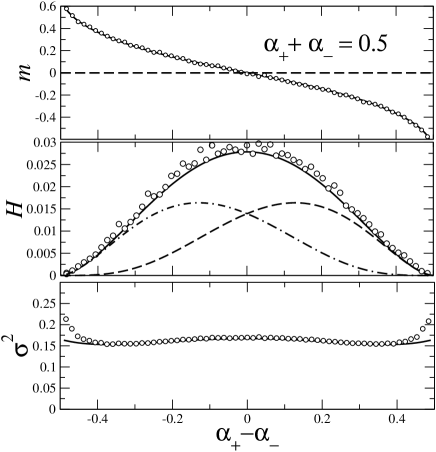
Figure 2: Behavior of $m$ (top), $H$ (middle) and $\sigma^{2}$ (bottom) versus $\alpha_{+}-\alpha_{-}$ for $\alpha_{+}+\alpha_{-}=0.5$. Markers correspond to simulations with $N=256$ agents, averaged over 200 disorder samples per point. Lines are analytical results (see Appendices A and B for details). In the middle panel, the dashed line corresponds to $H_{+}$ and the dot-dashed line corresponds to $H_{-}$.

A naïve argument would suggest that agents are attracted by information rich markets. Instead one sees that, in a range of parameters, agents play preferentially in the market with smaller information complexity $\alpha_{\gamma}$ and with the smallest information content $H_{\gamma}$. For all those traders with $|m_{i}|<1$, the conditions for the minimum of $H$ give

$$m_{i}=-\left\langle{a_{i+}^{\mu_{+}}A_{+}^{(-i)}}\right\rangle+\left\langle{a_{i-}^{\mu_{-}}A_{-}^{(-i)}}\right\rangle$$ (15)

where $A_{\gamma}^{(-i)}$ stands for the contribution to $A_{\gamma}$ of all traders except $i$. Hence $m_{i}$ equals the difference in the payoffs of agent $i$ against all other traders and this relation means that if $m_{i}>0$ then agent $i$ invests preferentially in asset $+$ because that is more convenient. Therefore, Fig. 2 implies that the relation between payoffs and information is less obvious than the naïve argument above suggests.

This somewhat paradoxical result is due to the fact that agents are constrained to trade in one of the two markets. Rather than seeking the most profitable asset, agents escape the asset where their loss is largest.

III Grand Canonical Minority Game with two assets

In the grand-canonical framework players have the option not to play if their expected payoff doesn’t beat a pre-determined benchmark (which represents for instance a fixed interest rate or an incentive to enter the market) GCMG . As in the previous case, we consider two assets or markets, tagged by $\gamma\in\{-1,1\}$ as before. Each trader disposes of one quenched random strategy $\bm{a}_{i\gamma}=\{a_{i\gamma}^{\mu_{\gamma}}\}$ per asset, which prescribes an action $a_{i\gamma}^{\mu_{\gamma}}\in\{-1,1\}$ for each possible information pattern $\mu_{\gamma}\in\{1,\ldots,P_{\gamma}\}$. Again $\mu_{\gamma}(t)$ are chosen at random independently for all $t$ and $\gamma=\pm 1$. As in the one-asset grand-canonical MG, it is necessary to introduce a certain number of traders – so-called producers – who invest at every time step no matter what. These can be regarded as traders with a fixed strategy $b_{i\gamma}^{\mu_{\gamma}}=\pm 1$. The number of producers in market $\gamma$ shall be denoted by $N_{p,\gamma}$ and their aggregate contribution to $A_{\gamma}(t)$ by $B_{\gamma}^{\mu_{\gamma}(t)}=\sum_{i=1}^{N_{p}}b_{i,\gamma}^{\mu_{\gamma}(t)}$. Therefore Eq. (2) becomes

$$A_{\gamma}(t)=\sum_{j=1}^{N}a^{\mu_{\gamma}(t)}_{j\gamma}\delta_{s_{j}(t),\gamma}+B_{\gamma}^{\mu_{\gamma}(t)}$$ (16)

The rest of the traders, the speculators, have an adaptive behavior which is again governed by the dynamics (1) but now agents can also decide not to trade. This choice is equivalent to trading in a fictitious $\gamma=0$ “asset” whose cumulated score is $U_{i,0}(t)=\epsilon t$. More precisely

$$s_{i}(t)={\rm arg}\max_{\gamma\in\{0,\pm 1\}}U_{i,\gamma}(t)$$ (17)

The $\gamma=0$ choice represents a fixed benchmark with a constant payoff. By Eq. (17) traders invest in $\gamma\not=0$ assets only if their score exceeds that of the benchmark, i.e. if the corresponding score $U_{i\gamma}$ grows at least as $\epsilon t$. Notice that agents are allowed to invest in at most one asset. If agents were allowed to invest in both $\gamma=\pm 1$ assets if $U_{i,\pm}(t)>U_{i,0}(t)$ then it is easy to see that the model becomes equivalent to two un-coupled GCMGs.

The arguments of the previous section show that also in this case no significant correlation between assets is introduced by the behavior of speculators. Again the collective properties of the stationary state can be characterized by the predictability $H$, Eq. (4), the volatility $\sigma^{2}$, Eq. (5) and the “magnetization” $m$ of Eq. (6). These parameters can be studied as before upon varying the parameters $\alpha^{\gamma}=P_{\gamma}/N$ and $\epsilon$. We also introduce the relative number of producers $n_{p}=N_{p,\gamma}/P_{\gamma}$, which for simplicity is assumed to be the same for both assets. Notice that for $n_{p}=0$ and $\epsilon\to-\infty$ we recover the model of the previous section where there are no producers and speculators are forced to trade.

We focus first on $m$ (see Fig. 3).

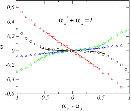
Figure 3: Behavior of $m$ versus $\alpha_{s}^{+}-\alpha_{s}^{-}$ for $\alpha_{s}^{+}+\alpha_{s}^{-}=1$ and flat initial conditions. Markers correspond to simulations with $N_{s}=200$ speculators, averaged over 200 disorder samples per point. Lines are analytical results (interrupted when the non-ergodic phase is met, see phase diagram). Other parameters are as follows: $\epsilon=0.1$, $n_{p}=1$ ($\diamond$); $\epsilon=0.1$, $n_{p}=0.1$ ($\bigtriangleup$); $\epsilon=-0.1$, $n_{p}=1$ ($\bigcirc$); $\epsilon=-0.1$, $n_{p}=0.1$ ($\square$).

One sees that when traders have positive incentives to trade ($\epsilon<0$) the market behaves as in the previous section, with speculators investing preferentially in the asset with less information. This tendency becomes less pronounced the larger is $n_{p}$, which is reasonable in view of our discussion above, because then the game becomes more and more profitable for speculators.

This scenario is qualitatively reproduced at all $\epsilon<0$ and it changes drastically as soon as $\epsilon>0$. In this case, traders concentrate most of their investments into the information-rich asset even if $n_{p}$ is very low. The fact that traders can refrain from investing implies that trading is dominated by gain seeking rather than escaping losses.

The theory for this case is slightly more involved than for the canonical model. On the static side, the Hamiltonian is now

$$H_{\epsilon}=\sum_{\gamma=\pm 1}\frac{1}{NP_{\gamma}}\sum_{\mu_{\gamma}=1}^{P_{\gamma}}\left[\sum_{j=1}^{N}a_{j\gamma}^{\mu_{\gamma}}\pi_{j}^{\gamma}+B_{\gamma}^{\mu_{\gamma}}\right]^{2}+\frac{2\epsilon}{N}\sum_{j=1}^{N}\pi_{j}^{0}$$ (18)

where $\pi_{i}^{\gamma}=\left\langle{\delta_{s_{i},\gamma}}\right\rangle$ denotes the frequency with which agent $i$ invests in asset $\gamma=0,\pm 1$ in the steady state. Notice that $H_{0}=H$ is the predictability. As before, it is necessary to introduce a fictitious temperature $\beta>0$ and turn to the replica trick to analyze the minima of $H_{\epsilon}$ over $\{\pi_{i}^{\gamma}\}$ considering the limit $\beta\to\infty$. The main difference with the canonical model lies in the fact that one must now consider an overlap order parameter per asset, namely $Q_{ab}^{\gamma}=(1/N)\sum_{i=1}^{N}\pi_{ia}^{\gamma}\pi_{ib}^{\gamma}$ ($a,b=1,\ldots,r$, $\gamma=\pm 1$) and, in the replica-symmetric Ansatz, one ‘susceptibility’ per asset, that is $\chi^{\gamma}=\beta(Q^{\gamma}-q^{\gamma})$.

Again these quantities can be given a dynamic interpretation with the generating function approach cool . This approach leads, in the batch approximation, to two effective processes (one per asset), namely

$$U_{\gamma}(\tau+1)=U_{\gamma}(\tau)-\epsilon+z_{\gamma}(\tau)\sqrt{1+\alpha_{\gamma}n_{p}}\\ -(1+\alpha_{\gamma}n_{p})\sum_{\tau^{\prime}}\left[\bm{1}+\lambda_{\gamma}\bm{G}_{\gamma}\right]^{-1}(\tau,\tau^{\prime})\phi_{\gamma}(\tau^{\prime})$$ (19)

where $\lambda_{\gamma}=\frac{1+\alpha_{\gamma}n_{p}}{\alpha_{\gamma}}$ and the noise correlations are described by the matrices $\Lambda_{\gamma}(\tau,\tau^{\prime})=\left\langle{z_{\gamma}(\tau)z_{\gamma}(\tau^{\prime})}\right\rangle$ with

$$\bm{\Lambda}_{\gamma}=\left[\left(\bm{1}+\lambda_{\gamma}\bm{G}_{\gamma}\right)^{-1}\left(\lambda_{\gamma}\bm{C}_{\gamma}\right)\left(\bm{1}+\lambda_{\gamma}\bm{G}_{\gamma}^{T}\right)^{-1}\right]$$ (20)

$$C_{\gamma}(\tau,\tau^{\prime})=\left\langle{\phi_{\gamma}(\tau)\phi_{\gamma}(\tau^{\prime})}\right\rangle~{}~{}~{}~{}~{}G_{\gamma}(\tau,\tau^{\prime})=\left\langle{\frac{\partial\phi_{\gamma}(\tau)}{\partial h_{\gamma}(\tau^{\prime})}}\right\rangle$$ (21)

In order to characterize time-translation invariant and ergodic steady states four quantities are now required, namely two persistent autocorrelations $q_{\gamma}=\lim_{\tau,\tau_{0}\to\infty}\frac{1}{\tau}\sum_{\tau^{\prime}=1}^{\tau}C_{\gamma}(\tau_{0},\tau_{0}+\tau^{\prime})$ and two susceptibilities $\chi_{\gamma}=\lim_{\tau,\tau_{0}\to\infty}\sum_{\tau^{\prime}=1}^{\tau}G_{\gamma}(\tau_{0},\tau_{0}+\tau^{\prime})$, $\gamma\in\{-1,1\}$. For these, one obtains equations that can be solved numerically and the quantity $m$ can be written in terms of the $q_{\gamma}$’s and the $\chi_{\gamma}$’s. Now ergodicity breaking is connected to the divergence of at least one of the susceptibilities.

The behavior of the model is considerably richer than in the previous case: For $\epsilon\not=0$ we find that $H_{\epsilon}$ has a unique non-degenerate minimum and both $\chi^{\gamma}$’s are finite. The case $\epsilon=0$ is peculiar as it marks the boundary between two different behaviors $\epsilon<0$ and $\epsilon>0$. For $\epsilon=0$ and $\alpha_{\pm}$ large enough, both markets are predictable ($H_{0}>0$) and the susceptibility is finite. However, one of the susceptibilities diverges while the other stays finite for lower values of $\alpha_{\pm}$. This signals the onset of a phase where one of the markets is unpredictable while still $H_{0}>0$, a situation with particularly striking dynamical consequences. As a result, the phase structure of this model is rather complex (see Fig. 4).

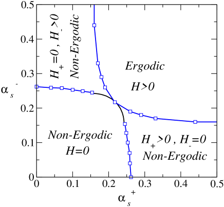
Figure 4: Phase diagram of the $\epsilon=0$, $n_{p}=1$ grand-canonical two-asset Minority Game in the $(\alpha_{s}^{+},\alpha_{s}^{-})$ plane. The continuous line is analytical, the other phase boundaries are obtained from numerical simulations (averages over 100 disorder samples per point).

We have been unable to obtain analytical lines for the complete phase structure at $\epsilon=0$. The phase boundary separating the region with $H=0$ from that with $H>0$ has been calculated assuming that both susceptibilities diverge keeping a finite ratio $\chi_{+}/\chi_{-}$. The phase boundary of the non-ergodic region (which would correspond to the divergence of just one of the susceptibilities) has been instead estimated from numerical simulations and the corresponding lines must be considered a crude approximation.

Fig. 5 shows the magnetization as a function of $\alpha_{+}-\alpha_{-}$ along the cut $\alpha_{+}+\alpha_{-}=0.4$ in the phase diagram. This line is entirely contained in the non-ergodic phase. While the market remains globally predictable ($H>0$) the fact that one of the markets becomes unpredictable (e.g. $H_{+}=0$) implies that the steady state depends on initial conditions.

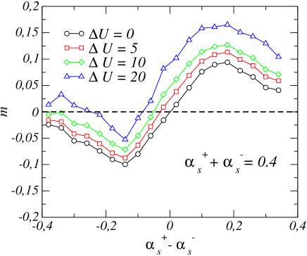
Figure 5: Behavior of $m$ versus $\alpha_{s}^{+}-\alpha_{s}^{-}$ for $\alpha_{s}^{+}+\alpha_{s}^{-}=0.4$, $\epsilon=0$, $n_{p}=1$ and biased initial conditions ($\Delta U=U_{i+}(0)-U_{i-}(0)$). Markers correspond to simulations with $N=200$ speculators, averaged over 200 disorder samples per point.

It is finally worth mentioning that the non-ergodic regimes with one unpredictable market extend to large values of $\alpha_{\gamma}$.

IV Conclusions

We have studied a multi-asset version of the Minority Game in order to address the problem of how adaptive heterogeneous agents would diversify their investments when the different assets bear different levels of information. While the phase structure of the models is substantially a generalization of that of single-asset games, we have found, in the grand-canonical model, a remarkable dependence of the probability to invest in a certain asset on the agent’s incentives to trade ($\epsilon$). Specifically, agents who have no incentives to trade other than the gains derived from it, invest preferentially in information-rich assets. On the contrary, when there are positive incentives to trade ($\epsilon<0$) agents invest more likely in the information-poor asset. This same behaviour is found in the canonical model, where agents must choose one asset at each time step and cannot refrain from entering the market.

The generalization of our results to a larger number of assets or to a wider strategy pool for the agents is straightforward. The results discussed here are indicative of the generic qualitative behavior we expect.

- (1) W. B. Arthur, Amer. Econ. Assoc. Papers and Proc. 84 406 (1994).
- (2) D. Challet and Y.-C. Zhang, Physica A 246 407 (1997).
- (3) D. Challet, M. Marsili and Y.-C. Zhang, Minority Games (Oxford University Press, Oxford, 2005).
- (4) A.C.C. Coolen, The mathematical theory of Minority Games (Oxford University Press, Oxford, 2005).
- (5) A. De Martino, M. Marsili and R. Mulet, Europhys. Lett. 65 283 (2004).
- (6) N. F. Johnson, P. M. Hui, D. F. Zheng and M. Hart, J. of Phys. A 32L427 (1999).
- (7) D. Challet and M. Marsili, Phys. Rev. E 68, 036132 (2003).
- (8) R. N. Mantegna, Eur. Phys. Jour. B 11, 193 (1999).
- (9) M. Potters, J. P. Bouchaud and L. Laloux, cond-mat/0507111 (2005).
- (10) J. P. Onnela, A. Chakraborti, K. Kaski, J. Kertesz, A. Kanto, Phys. Rev. E 68 (5) 056110 (2003).
- (11) R. D’Hulst and G. J. Rodgers, adap-org/9904003 (1999).
- (12) F. K. Chow and H. F. Chau, Physica A 319,601 (2003).
- (13) D. Challet, M. Marsili and R. Zecchina, Phys. Rev. Lett. 84 1824 (2000)
- (14) M. Marsili and D. Challet, Phys. Rev. E 64, 056138 (2001).
- (15) J.A.F. Heimel and A.C.C. Coolen, Phys. Rev. E 63 056121 (2001)