Averaged dynamics of two-phase media in a vibration field

Abstract

The averaged dynamics of various two-phase systems in a high-frequency vibration field is studied theoretically. The continuum approach is applied to describe such systems as solid particle suspensions, emulsions, bubbly fluids, when the volume concentration of the disperse phase is small and gravity is insignificant. The dynamics of the disperse system is considered by means of the method of averaging, when the fast pulsation and slow averaged motion can be treated separately. Two averaged models for both nondeformable and deformable particles, when the compressibility of the disperse phase becomes important, are obtained. A criterion when the compressibility of bubbles cannot be neglected is figured out. For both cases the developed models are applied to study the averaged dynamics of the disperse media in an infinite plane layer under the action of transversal vibration.

I Introduction

Oscillatory processes can be found in a sheer uncountable number of situations in nature at various time and length scales: from subatomic to astronomic scales. Vibration is a mechanical oscillatory process with an amplitude small compared to the characteristic length scale of the system. Often, as in our study, it is assumed that the inherent time scale of the system is much larger than the period of the oscillation. Vibration mechanics has been studied for a long time, general concepts of this nonlinear phenomenon have been put into practice. It is widely used in industry for transportation and separation of granular matter such as powders and grains, to enhance mixing and reaction rates of different species. In medicine, ultrasound is applied for diagnostics and healing. In microfluidics and biotechnology it serves as a means to manipulate physical (colloidal particles, fine-dispersed powders, liquid drops in microemulsions) and biological (cells, microorganisms, and micromolecules) objects suspended in liquids. Quite a broad spectrum of applications has motivated a great interest in the fundamental problems of vibration dynamics. The present work is aimed at studying the dynamics of two-phase media in a high-frequency vibration field.

There has been much effort to understand the impact of vibration action on the behavior of systems of different nature. Particularly, it has been understood that vibration can substantially influence the dynamic and rheologic properties of systems. An outstanding example is the Kapitza pendulum with a periodically moving point of support, kapitza-51 where the upper vertical state of the pendulum becomes stable. Other known effects are a metal ball that lifts in ambient sand medium under vibration, blekhman-00 granular matter that liquidizes evesque-rajchenbach-89 or demonstrates the formation of oscillons umbanhowar-etal-96 in a vibration field. As typical hydrodynamic examples we mention excitation of a steady relief at the oscillating interface pure liquid–particle suspension, ivanova-etal-96 ; lyubimov-etal-99 and thermal vibration convection, lyubimov-gersguni-98 where the action of vibration on the nonuniform fluid results in generation of a slow macroscopic motion even in the absence of gravity.

The behavior of a single solid inclusion in fluid environment under vibration has attracted much attention since long time ago. As far back as 1831, Faraday used particles to visualize standing acoustic waves and observed the effect of particle localization in the acoustic field.faraday-1831 The dynamics of a solid particle suspended in a vertically oscillating fluid was studied in Ref. boyadzhiev-73, . It was shown that vibration results in an average force, which can be used to affect particle dynamics. Granat granat-60 considered theoretically a motion of a solid sphere in a periodically oscillating flow of a viscous fluid. For the fluid with the density higher than that of the sphere, the latter oscillates with a smaller amplitude and a lag in phase. Conversely, in a relatively less dense fluid the oscillation of the sphere occurs with a larger amplitude with respect to the flow and leads in phase. In an experimental study by Chelomey,chelomey-83 the behavior of solid bodies in a vertically vibrated vessel with a fluid was investigated. It was observed that under vibration action, bodies with higher than ambient density could rise to the surface, whereas light bodies could sink. Theoretically, the averaged behavior of a solid sphere suspended in oscillated fluid near a wall was discussed in Ref. lamb-75, and has been recently generalized.lugovtsov-sennitskii-01 ; lyubimov-etal-01 It has been demonstrated that in addition to the gravity and Archemedian forces there appears an averaged force that attracts the body to the wall due to vibration. This vibration force can lead to ascent of heavy or settling down of light bodies, as was observed experimentally. chelomey-83

The dynamics of a single compressible bubble in vibration fields has been studied by many authors. The first analysis of the bubble dynamics was made by Rayleigh rayleigh-17 (see also Ref. lamb-75, ). A nonlinear equation that couples the radius of a bubble to the pressure in the liquid at large distance from the bubble, known as the Rayleigh-Plesset or Rayleigh-Lamb equation, was obtained and the eigenfrequencies of the small oscillations were determined. Since then, many important aspects of nonlinear bubble dynamics and cavitation hasve been studied, e.g., natural and forced oscillations, parametric instability, which causes the oscillation of the bubble shape against a background of spherical pulsation, the influence of heat exchange between bubbles and ambient fluid and nonideality of the gas filling the bubble, the behavior of bubbles in nonuniform flows (see reviews in Refs. plesset-prosperetti-77, ; feng-leal-97, ).

In the context of the time-averaged dynamics of a bubble an important problem is obtaining the force exerted on the bubble due to vibration. The behavior of a single bubble in a standing acoustic wave is determined by “the primary Bjerknes force” after Bjerknes, bjerknes-06 who proposed its qualitative explanation. The effect is quite general: the bubbles migrate to the nodes of the pressure wave at high frequencies $\omega>\omega_{0}$ and to antinodes at low frequencies $\omega<\omega_{0}$, where $\omega_{0}$ is the frequency of natural oscillation of the bubble. The average force on a particle, called the force of radiation pressure, was obtained by Yosioka and Kawasima.yosioka-kawasima-55 The considered setup comprised a liquid drop in another liquid in a standing acoustic wave, where both liquids were assumed to be compressible. A generalization for the case of an arbitrary nonuniform oscillating flow has been provided by Alekseev.alekseev-83 These results can be applied to analyze both limiting cases – the primary Bjerknes effect for deformable bubbles and the behavior of a solid particle in nonuniform pulsating flows.

Generalization of the description of a separate particle suspended in a fluid to the case of a disperse medium (ensemble of many particles) requires space averaging. The precise description of all the disperse particles becomes redundant and unfeasible. There are basically three possibilities to obtain a reasonable model: (i) statistical approach, concerned with averaging over the ensemble of particles; for solid particles and bubbles such a procedure is carried out in Refs. zhang-prosperetti-JFM-94, ; zhang-prosperetti-PhF-94, ; bulthuis-etal-95, ; (ii) derivation of a kinetic equation (see, e.g., Refs. smereka-96, ; russo-smereka-I-96, ; teshukov-gavrilyuk-02, ); (iii) continuum models, where after the space-averaging the disperse particles are treated as a separate continuum.wijngaarden-72 ; nigmatulin-91 In our study, we apply the last approach.

Although, wave propagation in disperse media is well understood, the problem of the time-averaged dynamics for such systems has received relatively little attention and remains rather unexplored. Most of studies deal with acoustic vibration, when the compressibility of carrier fluid is of crucial importance; the feedback of particles on the flow is conventionally neglected. For instance, Ganiev and Lapchinskyganiev-lapchinsky-78 studied averaged collective behavior of bubbles and solid particles suspended in fluids in acoustic fields. The analog of the primary Bjerknes effect was observed and simple explanation was provided. In the present study, we concentrate on the averaged effects in various disperse media under the action of high frequency, but subacoustic vibration field, i.e., when the fluid is incompressible. We also take into account the feedback of particles on the carrier fluid and demonstrate that this is an important factor, which can lead to nontrivial effects.

The paper is outlined as follows. In Sec. II the theoretical model is developed for a suspension of nondeformable particles. The equations describing the pulsation and averaged dynamics are obtained. On the basis of this model the stability of a quasiequilibrium state in a plane layer is analyzed in Sec. III. Section IV addresses the vibrational dynamics of bubbly fluids. An averaged model accounting for the compressibility of bubbles is obtained. Particularly, it is shown that in the limit of weak compressibility this model reduces to the model for nondeformable particles, obtained in Sec. II. In Sec. V, the developed model is applied to investigate the dynamics of a bubbly fluid in a plane layer under vibration action. The results are summarized in Sec. VI.

II Theoretical model of a nondeformable particle suspension in a vibration field

II.1 Governing equations and basic assumptions

Consider the behavior of an isothermal fluid (liquid or gas) laden with disperse particles (solid particles, small droplets of another liquid or bubbles) under the action of high frequency vibration. We assume that all the particles are monodisperse spheres of a radius $r_{d}$ and the amplitude of vibration $a$ is small compared to this size: $a\ll r_{d}$ (for viscous pulsation a milder restriction is enough to be held, see Sec. II.2). The frequency of vibration $\omega$ is assumed to be so high that the size of a viscous boundary layer $\ell=\sqrt{\nu/\omega}$ ($\nu$ is the kinematic viscosity of the fluid) near the walls of a container with the suspension is small with respect to the characteristic scale $L$ of a flow. On the other hand, the scale $L$ is considered to be small compared to the acoustic wave length $\lambda_{a}=2\pi v_{a}/\omega$ ($v_{a}$ is the acoustic speed), which leads to a twofold inequality $\nu/L^{2}\ll\omega\ll v_{a}/L$.

We start with a two-fluid model valid for dilute suspensions, when one can neglect interparticle interactions and interactions between the particles and walls of a container. We assume that the size $r_{d}$ is large enough to neglect diffusion of particles, but small with respect to $L$. On a scale much greater than $r_{d}$ the particles are regarded as a continuum with the volume fraction $\varphi=4/3\pi r_{d}^{3}n$ (the volume fraction of the fluid phase is $1-\varphi$), where $n$ is the number of particles per unit volume of the medium. It is also supposed that the particles can neither deform nor combine into agglomerates; the carrier and the disperse phases have constant densities $\rho$ and $\rho_{d}$ (hereafter, the subscript “$d$” stands for the disperse phase). Since $\varphi$ differs from $n$ by a constant factor, in the following $\varphi$ is called concentration. After averaging over space the equations for mass and momentum of the phases read:nigmatulin-91

$${\rm div}\left(1-\varphi\right){\bf U}+{\rm div}\,\varphi{\bf U}_{d} = 0,$$ (1a)

$$\frac{d\varphi}{dt}+\varphi\,{\rm div}\,{\bf U}_{d} = 0,$$ (1b)

$$\left(1-\varphi\right)\rho\frac{D\bf U}{Dt} = -\nabla P+\mu\nabla\cdot\left(1-\varphi\right){\bf\varepsilon}-\varphi{\bf F},$$ (2a)

$$\rho_{d}\,\frac{d{\bf U}_{d}}{dt} = {\bf F},$$ (2b)

where ${\bf U}$ and ${\bf U}_{d}$ are the velocities of the phases, $P$ is the pressure in fluid, $\mu$ is the fluid viscosity, the shear rate tensor is given by $\varepsilon_{ij}=\nabla_{i}U_{j}+\nabla_{j}U_{i}$. Derivatives $D/Dt=\partial/\partial t+{\bf U}\cdot\nabla$ and $d/dt=\partial/\partial t+{\bf U}_{d}\cdot\nabla$ are taken along the Largangian path of the elements of the fluid and the disperse phase, respectively.

The interphase interaction force can be written as follows:nigmatulin-91 ; maxey-riley-83 ; yang-leal-91

$${\bf F} = \rho\frac{D\bf U}{Dt}-\frac{9}{2r_{d}^{2}}\left(\frac{2/3+\kappa}{1+\kappa}\right){\bf W}$$ (3)

$$-\frac{9}{2r_{d}}\left(\frac{\kappa}{1+\kappa}\right)\sqrt{\frac{\rho\mu}{\pi}}\int\limits_{0}^{t}\frac{d{\bf W}(\zeta)}{d\zeta}\frac{d\zeta}{\sqrt{t-\zeta}}$$

$$-\frac{1}{2}\rho\frac{d{\bf W}}{dt}-{\bf F}_{m}.$$

Here, the relative velocity of phases ${\bf W}={\bf U}_{d}-{\bf U}$ and the ratio of viscosities of phases $\kappa=\mu_{d}/\mu$ are introduced. The first term in (3) is a force due to pressure gradient, the next forces are the Stokes (Hadamard-Rybczynski) drag, lamb-75 and three unsteady forces: the Basset history force, the added mass force, allowing for the inertia of the surrounding fluid, and a second memory force that is essential for non-solid particles. yang-leal-91 We do not consider the effects that can be initiated by rotation of particles, therefore the Magnus force is not taken into account.

The relative contribution of the Stokes drag $F_{S}$, the Basset $F_{B}$, and the added mass $F_{M}$ forces to the interphase force (3) is governed by an “unsteadiness parameter” $K=r_{d}/\sqrt{\nu t_{*}}$:

$$\frac{F_{B}}{F_{S}}\sim K,\quad\frac{F_{M}}{F_{S}}\sim K^{2},$$

where $t_{*}$ is the timescale of the variation of the relative velocity of phases. Note, that the pressure gradient term and the added mass force in (3) are of the same order. The same argument can be applied to the memory forces, except for the limiting cases of an inviscid bubble ($\kappa=0$) and a solid particle ($\kappa\gg 1$), when, either the Basset term or the second memory force vanish, respectively.

For quasisteady flows ($K\ll 1$) and the flow regimes with finite $K$, the result (3) holds provided that the particle Reynolds number ${\rm Re}_{d}$ is small and gradients of the velocity ${\bf U}$ are not too large: maxey-riley-83

$${\rm Re}_{d}=\frac{r_{d}W}{\nu}\ll 1,\quad\frac{r_{d}^{2}\,U}{\nu L}\ll 1.$$ (4)

In the case of substantially unsteady flows ($K\gg 1$), the force (3) has inviscid nature and the validity criterion does not depend on the viscosity. The restrictions (4) should be replaced with the conditions

$$\frac{Wt_{*}}{r_{d}}\ll 1,\quad\frac{Ut_{*}}{L}\ll 1,$$ (5)

which arise from linearization requirements. Note, that in this limit, $Re_{d}$ is not necessarily small and for finite and large $Re_{d}$ the forces depending on viscosity in expression (3) have to be modified. clift-etal-78 However, for the flow with $K\gg 1$, these terms (irrespective of the modification) are small compared to the leading pressure gradient and added mass forces and therefore can be neglected.

The governing equations are formulated in an inertial reference frame; the influence of vibration should be taken into account through boundary conditions.

II.2 Pulsation velocities

The presence of two considerably different time scales, namely, the characteristic oscillation time $1/\omega$ and the dissipative time scale $L^{2}/\nu$, makes reasonable to use the multiscale technique:nayfeh-81 the “fast” and the “slow” averaged motions are treated separately. So, the operator of time differentiation is replaced by a sum of two operators $\partial/\partial t\to\omega\,\partial/\partial\tau+\partial/\partial t$, where $\tau=\omega t$ is the fast time; the actual fields of the velocities, the pressure, and the concentration are represented by sums of the averaged (over the fast time $\tau$) and the fast, or pulsation, components, respectively: ${\bf U}={\bf u}+{\bf V}$, ${\bf U}_{d}={\bf u}_{d}+{\bf V}_{d}$, $P=p+q$, $\varphi=c+\phi$.

Let us substitute this ansatz into the governing equations and obtain the pulsation parts of the momentum Eqs. (2). We retain only the leading terms and take into account a smallness of the concentration pulsation, $\phi\sim(a/L)c$, which follows from Eq. (1b). The dimensionless variables are introduced using the following units: $1/\omega$ and $L^{2}/\nu$ for the fast and the averaged time, $a\omega$ and $\nu/L$ for the pulsation and the averaged velocities of the phases, $\rho a\omega^{2}L$ and $\rho\nu^{2}/L^{2}$ for the pulsation and the averaged pressure, respectively. It is assumed that the space derivatives can be evaluated with the scale $L$, which means that the small scale dynamics in boundary layers near solid walls and turbulent pulsations are not considered. As a result, we arrive at the equations for the fast dynamics:

$${\rm div}(1-c){\bf V}+{\rm div}\,c{\bf V}_{d} = 0,$$ (6a)

$$\frac{\partial\phi}{\partial\tau}+{\rm div}\,c{\bf V}_{d} = 0,$$ (6b)

$$\frac{\partial{\bf V}}{\partial\tau} = -\nabla q+c\,{\bf f},$$ (7a)

$$\delta\frac{\partial{\bf V}_{d}}{\partial\tau} = \frac{\partial{\bf V}}{\partial\tau}-{\bf f},$$ (7b)

$${\bf f} = \frac{1}{K^{2}}\left(\frac{2/3+\kappa}{1+\kappa}\right){\bf w}$$ (8)

$$+\frac{1}{K\sqrt{\pi}}\left(\frac{\kappa}{1+\kappa}\right)\int\limits_{0}^{\tau}\frac{\partial{\bf w}(\zeta)}{\partial\zeta}\frac{d\zeta}{\sqrt{\tau-\zeta}}$$

$$+\frac{1}{2}\frac{\partial{\bf w}}{\partial\tau}+{\bf f}_{m},$$

where the relative pulsation velocity ${\bf w}={\bf V}_{d}-{\bf V}$ and a dimensionless parameter $\delta=\rho_{d}/\rho$, which is the ratio of densities of the phases, are introduced; the pulsation component of the memory force ${\bf F}_{m}$ is denoted by ${\bf f}_{m}$. For the case of pulsation motion, the unsteadyness parameter $K=r_{d}/\ell$ has the meaning of the ratio of the particle radius to the size of a viscous boundary layer around it.

The restrictions for the amplitude of vibration $a$ are imposed by the inequalities (4), (5), and the necessity of linearization of the pulsation problem (6)-(8). For the motion with finite $K$ and in the limit of inviscid pulsations, $K\gg 1$, the vibration amplitude is required to be small in the sense $a\ll r_{d}$. However, in the limit of viscous pulsation, $K\ll 1$, a much milder restriction for the vibration amplitude is enough to be held: $a\ll\min\left(L,K^{-2}r_{d}\right)$.

Let us restrict our consideration to the case of the monochromatic vibration and proceed to complex amplitudes: $\mathscr{F}({\bf r},t)={\rm Re}\left[\hat{\mathscr{F}}({\bf r})\exp(i\tau)\right]$. For such a vibration process, ${\bf\hat{f}}$ coincides (in dimensionless form) with the Fourier-transform of the pulsation force ${\bf f}$ and can be represented as (cf. Refs. yang-leal-91, ; kim-karrila-91, ):

$$\hat{\bf f}=\chi\hat{\bf w},$$ (9)

$$\chi=\frac{9}{2K^{2}}\left(1+\lambda+\frac{\lambda^{2}}{9}\right.$$

$$\left.-\frac{(1+\lambda)^{2}f(\lambda)}{\kappa\left[\lambda^{3}-\lambda^{2}\tanh\lambda-2f(\lambda)\right]+(\lambda+3)f(\lambda)}\right),$$ (10)

where $\lambda=(1+i)K/\sqrt{2}$ and $f(\lambda)=\lambda^{2}\tanh\lambda-3\lambda+3\tanh\lambda$.

As follows from Eqs. (6), (7) and relation (9), the pulsation velocities are not independent, therefore the problem can be expressed in terms of an auxiliary field ${\bf v}=(1-c){\bf\hat{V}}+c{\bf\hat{V}}_{d}$ having the meaning of the amplitude of the volume-weighted velocity of the medium:

$$\nabla\times S\,{\bf v}=0,\quad{\rm div}\,{\bf v}=0,$$ (11)

$$S=\frac{\chi\rho_{m}+i\delta}{\chi+i\delta/\rho_{e}},$$ (12)

where $\rho_{m}=1-c+c\delta$ is the density of the medium and $1/\rho_{e}=1-c+c/\delta$ is the specific volume. The pulsation velocities expressed in terms of ${\bf v}$ are as follows:

$$\hat{\bf V} = \frac{\chi+i\delta}{\chi+i\delta/\rho_{e}}{\bf v},$$ (13)

$$\hat{\bf V}_{d} = \frac{\chi+i}{\chi+i\delta/\rho_{e}}{\bf v}.$$ (14)

Note, that except for the limiting cases of viscous ($K\ll 1$) and inviscid ($K\gg 1$) vibration regime, there appears a phase shift in the pulsation velocities of the particles and carrier fluid.

Now restrict our theory to the case of a closed nondeformable cavity, filled entirely with the two-phase medium. Equations (11) should be supplemented with the boundary conditions. The smallness of the vibration amplitude allows us to prescribe the boundary conditions at the average position. Because of incompressibility of the medium, the normal component of the velocity ${\bf v}$ has to coincide with that of the boundary velocity ${\bm{\xi}}$ at every point of the boundary $\Gamma$:

$${\bf n}\cdot{\bf v}|_{\Gamma}={\bf n}\cdot{\bm{\xi}},$$ (15)

where ${\bf n}$ is the unit normal to the average position of the boundary.

Assume that the system is subjected to translational, linearly polarized vibration. In this case the boundary velocity of the cavity is a constant vector: ${\bm{\xi}}={\bf j}$ (${\bf j}$ is the unit vector aligned along the vibration axis).

Since the particle concentration is small, the solution to the pulsation problem (11), (15) is sought as a series in $c$: ${\bf v}={\bf v}_{0}+{\bf v}_{1}+\ldots$ with ${\bf v}_{1}\sim c$ (and analogously for $\hat{\bf V}$, $\hat{\bf V}_{d}$). Then, to the leading order we obtain

$${\bf v}_{0}=\hat{\bf V}_{0}={\bf j},$$ (16)

i.e., the pulsation field is constant in the entire cavity: uniform fluid moves together with the cavity as a solid. Hence, to this approximation, the vibration does not influence the system, therefore it is necessary to obtain a nonuniform correction to the pulsation field.

Taking into account Eqs. (11), (15) and the result (16), to the next order we arrive at a problem

$$\nabla\times{\bf v}_{1} = S_{1}\,{\bf j}\times\nabla c,\quad{\rm div}\,{\bf v}_{1}=0,$$ (17)

$${\bf n}\cdot{\bf v}_{1}|_{\Gamma} = 0,$$

$$S_{1} = \left(\delta-1\right)\frac{\chi+i}{\chi+i\delta},$$

where $S_{1}$ is a coefficient in a corresponding expansion of (12): $S=1+S_{1}\,c+O(c^{2})$. It becomes clear from Eq. (17), that a nonuniformity of the pulsation field ${\bf v}_{1}$ is caused by interaction of vibration with inhomogenieties in the particle concentration. We make a note, that an explicit solution for the field ${\bf v}_{1}$ is not needed while obtaining the averaged equations of motion: only the vorticity and divergency of ${\bf v}_{1}$ are further used.

II.3 Averaged equations. Single-fluid approximation

We now turn to averaging of the governing equations. Let us write out the averaged parts of Eqs. (1), (2) and retain only the leading terms. Note, that averaged dynamics can be described in terms of a single-fluid model. Contrastingly to the pulsation motion, relative contributions of the Stokes drag, the memory forces, and the added mass force to the averaged dynamics are defined by a small parameter $r_{d}/L$; the unsteady forces turn out to be small compared with the Stokes force and therefore can be neglected. Because the difference in the averaged velocities of the phases ${\bf u}_{d}-{\bf u}$ is of order $r_{d}^{2}/L^{2}$, we neglect it everywhere, except for the interphase force. In the latter, this difference must be retained: despite its smallness, it is multiplied by a vibration parameter $\tilde{R}_{v}=a^{2}\omega^{2}L^{2}/\nu^{2}$, which can be large, and a corresponding contribution in the averaged equations is generally finite. As a result, we obtain the following equation of motion

$$\rho_{m}\left(\frac{\partial{\bf u}}{\partial t}+{\bf u}\cdot\nabla{\bf u}\right) + \tilde{R}_{v}\nabla\cdot\left[\left(1-c\right)\overline{{\bf V}{\bf V}}+\delta c\overline{{\bf V}_{d}{\bf V}_{d}}\right]$$ (18)

$$= -\nabla p+\nabla\cdot\left(1-c\right)\varepsilon.$$

Here, $\varepsilon$ is the averaged shear rate tensor; overlines are used to denote averaging over time. The accepted approximation means, that the particles are “frozen” in the averaged carrier flow.

It is important to note, that the nonuniformity of the pulsation field can be caused not only by the considered mechanism, when vibration interacts with nonuniformity of the medium due to admixture. Another reason for a nonuniformity in the pulsation field is interaction of vibration with the vorticity of the averaged flow. A contribution to the averaged equations due to the second mechanism is defined by the vector of pulsation transport (see discussion in Ref. lyubimov-gersguni-98, ). However, for the linearly polarized vibration, the case under consideration, this vector vanishes. A quite similar situation takes place in thermal vibrational convection.lyubimov-gersguni-98 The only difference is that there the nonuniformity of density is caused by nonisothermality of fluid, but not due to the presence of a disperse phase.

Using (13), (14), we calculate the averaged Reynolds stress

$$\left(1-c\right)\overline{{\bf V}{\bf V}}+\delta c\overline{{\bf V}_{d}{\bf V}_{d}}=G\,{\rm Re}\left({\bf v}{\bf v}^{\ast}\right),$$ (19)

$$G = \frac{1}{2}(1-c)\left|\frac{\chi+i\delta}{\chi+i\delta/\rho_{e}}\right|^{2}+\frac{1}{2}\delta c\left|\frac{\chi+i}{\chi+i\delta/\rho_{e}}\right|^{2}.$$ (20)

Taking into account smallness of the particle concentration, the result (16), and Eqs. (11), we evaluate the “vibration force”

$$\tilde{R}_{v}\nabla\cdot\left[G\,{\rm Re}\left({\bf v}{\bf v}^{\ast}\right)\right] = -\tilde{R}_{v}B\,{\bf j}\,{\bf j}\cdot\nabla c+\ldots,$$

$$B = \frac{\left(\delta-1\right)^{2}{\rm Im}\chi}{2\left|\chi+i\delta\right|^{2}},$$ (21)

where dots denote the omitted gradient terms. Such terms lead only to a renormalization of the pressure, which is not important in the framework of our consideration.

In the vein of the Boussinesq approximation, we neglect the nonuniformities of the density everywhere except for the the vibration force, where the small concentration is multiplied by the vibration parameter $\tilde{R}_{v}$, which is generally large. Such a transformation corresponds to a limiting transition, when $\tilde{R}_{v}\to\infty$, $c\to 0$, but their product $\tilde{R}_{v}c_{\ast}$ is finite (here $c_{\ast}$ is the reference value of the particle concentration).

Averaging of the mass balance equations is straightforward. Finally, we end up with a set of the averaged equations describing the behavior of a suspension of nondeformable particles in a high frequency vibration field:

$$\frac{\partial{\bf u}}{\partial t}+{\bf u}\cdot\nabla{\bf u}-R_{v}\,{\bf j}\,{\bf j}\cdot\nabla c = -\nabla\Pi+\nabla^{2}{\bf u},$$ (22)

$$\frac{\partial c}{\partial t}+{\bf u}\cdot\nabla c = 0,\quad{\rm div}\,{\bf u}=0,$$ (23)

where $\Pi$ is the renormalized pressure, the concentration is normalized by $c_{\ast}$, and the vibration parameter is redefined $R_{v}=a^{2}\omega^{2}L^{2}Bc_{\ast}/\nu^{2}$.

The vibration force, appeared as a result of averaging of the equations, is caused by interaction of the monochromatic linearly polarized vibration with the inhomogeneity of medium due to a nonuniform distribution of particles; for the uniform distribution of particles it vanishes. The force is directed along the vibration axis and takes on maximal values in the domains of the flow where the gradient of particle concentration coincides with the direction of the vibration axis. For the initial state with a nonuniform distribution of particles and the vanishing averaged velocity the action of the vibration force can result in generation of averaged motion.

It is important to make a note of the generic character of the vibration force. The dependence on the parameters $\delta$, $\kappa$, $K$, i.e., on the the nature of the particles, is gathered in the parameter $B$. This allows us to make two conclusions. First, since $B>0$ for all values of these parameters, the direction of the force is determined only by the concentration field and an orientation of the vibration axis. Second, for different media only the intensity of response towards vibration action changes. However, such a quantitative distinction is worth discussing for comparison with experiments, therefore properties of the function $B=B(\delta,\kappa,K)$ are discussed in Appendix.

The set of averaged Eqs. (22), (23) must be supplemented with boundary conditions for the velocity. For the considered case of vibration action, the Schlichting mechanism schlichting-68 of surface generation of averaged flow is absent, therefore on a rigid surface $\Gamma$ one should use the conventional no-slip boundary condition

$${\bf u}|_{\Gamma}=0.$$ (24)

Indeed, the intensity of the averaged flow caused by the Schlichting mechanism is governed by the pulsation Reynolds number lyubimov-gersguni-98 ${\rm Re}_{p}=a^{2}\omega/\nu$. Compared to the considered bulk mechanism, which is governed by the parameter $R_{v}$, the Schlichting mechanism can give a finite contribution to generation of averaged motion only if the leading part of the pulsation velocity is nonuniform. In our case, this requirement is not satisfied: according to (16), the leading part of the pulsation velocity is uniform, a nonuniformity occurs only as a small correction to the uniform term. Hence, the Schlichting generation of averaged flow is negligible compared to the contribution of the bulk mechanism. Rather similar situation takes place in thermal vibration convection: for the same kind of vibration action on weakly nonuniform fluid, when the density nonuniformity is caused by nonisothermality of fluid, the Schlichting mechanism does not contribute to generation of average flow.

III Stability of a quasiequilibrium in vibration field

III.1 Basic quasiequilibrium state

Let a suspension fill an infinite plane layer $-1<z<1$ (of a dimensional width $2h$) in weightlessness. Consider the influence of the transversal linearly polarized vibration on the stability of a quasiequilibrium. A quasiequilibrium is thought of as a state in which the averaged velocity vanishes in the entire volume of the system, whereas the pulsation velocity is different from zero.

This problem is described by Eqs. (22), (23) with ${\bf j}=(0,0,1)$ and boundary conditions (24). By setting ${\bf u}=0$ in the equations, we obtain the conditions defining the quasiequilibrium state

$$R_{v}{\bf j\,j}\cdot\nabla c_{0}=\nabla\Pi_{0},\quad c_{0}={\rm const}(t),$$

where the subscript “0” indicates the state of quasiequilibrium. Integration of the first equation leads to a condition

$$R_{v}c_{0}(x,y,z)=\Pi_{0}(z)+f(x,y).$$ (25)

Here $f(x,y)$ is an arbitrary function of longitudinal coordinates. Thus, there is a set of possible quasiequilibrium distributions of particles that is defined by a sum of a function of only transversal coordinate and a function of longitudinal coordinates.

As a quasiequilibrium concentration we choose a linear function of the transversal coordinate

$$c_{0}=\alpha+\beta z,\quad\alpha>0,\quad|\beta|<\alpha$$ (26)

and investigate its stability. Although gravity is unimportant in the framework of our theory, in a quiescent fluid (in the absence of vibration) it ultimately leads to stratification of particles. For this reason, the choice of the initial distribution of particles in the form (26) is rather natural for a narrow layer. Further, as a reference value for the particle concentration we use $\beta h$, therefore $R_{v}=a^{2}\omega^{2}h^{3}B\beta/\nu^{2}$.

III.2 Statement of linear stability problem

To investigate the stability of the quasiequilibrium state we introduce perturbations of the velocity ${\bf u}$, the pressure $q$, and the concentration $\phi$ , and substitute the disturbed fields ${\bf u}$, $\Pi_{0}+q$, $c_{0}+\phi$ into the problem (22)-(24). We linearize the equations near the quasiequilibrium and obtain a set of equations and boundary conditions for small perturbations

$$\frac{\partial{\bf u}}{\partial t}-R_{v}\,{\bf j}\,{\bf j}\cdot\nabla\phi = -\nabla q+\nabla^{2}{\bf u},$$

$$\frac{\partial\phi}{\partial t}+{\bf u}\cdot\nabla c_{0} = 0,\quad{\rm div}\,{\bf u}=0,$$

$$z = \pm 1:\;{\bf u}=0.$$

Since the quasiequilibrium state is uniform and isotropic in a plane of the layer, we can restrict our stability analysis to the case of the two-dimensional perturbations in the form of rolls. Assuming all the perturbations to be proportional to $\exp(\lambda t-iky)$, where $\lambda=\lambda_{r}+i\lambda_{i}$ is the complex growth rate and $k$ is the real wave number, we rewrite the problem for one variable. Eliminating the pressure from the equation of motion and taking into account the continuity equation, we obtain for the amplitude $\hat{\phi}$ of the concentration perturbation (the perturbations of the concentration and the transversal component of the velocity differ only by a constant factor):

$$\lambda^{2}D^{2}\hat{\phi}-R_{v}k^{2}\hat{\phi}^{\prime}=\lambda D^{4}\hat{\phi},$$ (27)

$$z=\pm 1:\;\hat{\phi}=0,\;\hat{\phi}^{\prime}=0,$$ (28)

where a differential operator $D^{2}=d^{2}/dz^{2}-k^{2}$ is introduced. While obtaining (27), (28) it was assumed that $\lambda\neq 0$. In the opposite case, $\lambda=0$, there exist obvious solutions $\hat{\phi}={\rm const}$ for $k\neq 0$ and $\hat{\phi}=\hat{\phi}(z)$ for $kR_{v}=0$; the perturbations of the velocity vanish for both these cases. The existence of these neutrally stable solutions is easy to explain: although the mentioned perturbations deform the concentration field (26), it still belongs to the set of quasiequilibrium solutions (25).

The boundary value problem (27), (28) is a spectral amplitude problem, the condition of nontrivial solution defines the growth rate $\lambda$ as a function of parameters $R_{v}$, $k$. In the absence of vibration ($R_{v}=0$), besides the discussed solutions for $\lambda=0$, the problem admits an explicit solution, gershuni-zhuhovitsky-76 eigenvalues of which belong to a spectrum of real negative values: all the perturbations decay and the system is stable. Further we are interested in the nontrivial case of $R_{v}\neq 0$. In this case the problem (27), (28) is no longer self-adjoint, therefore the spectrum of growth rates can be complex.

Because the parameter $\beta$ is not of the fixed sign, the vibration parameter can take on both positive and negative values. However, the problem is invariant with respect to the mutual change of sign of the transversal coordinate and the vibration parameter. Such a symmetry is caused by the absence of gravity, which allows us to restrict our analysis to the case $R_{v}>0$.

III.3 The case of small values of vibration number $R_{v}$

Consider the case of small intensities of vibration action. We look for a solution to the problem (27), (28) in the form of series in small $R_{v}$

$$\hat{\phi}=\hat{\phi}_{0}+R_{v}\hat{\phi}_{1}+R_{v}^{2}\hat{\phi}_{2}+\ldots,\quad\lambda=\lambda_{0}+R_{v}\lambda_{1}+R_{v}^{2}\lambda_{2}+\ldots.$$ (29)

Substituting these expansions into Eqs. (27), (28), we find that $\hat{\phi}_{0}$ and $\lambda_{1}$ are defined by the following problem

$$\lambda_{1}D^{4}\hat{\phi}_{0}+k^{2}\hat{\phi}^{\prime}_{0}=0,$$ (30)

$$\hat{\phi}_{0}(\pm 1)=0,\;\hat{\phi}_{0}^{\prime}(\pm 1)=0.$$ (31)

Let us multiply Eq. (30) by the complex conjugate $\hat{\phi}_{0}^{\ast}$ and integrate by parts across the layer. Taking into account (31), after straightforward transformation we recognize that $\lambda_{1}=i\omega_{1}$, where $\omega_{1}$ is a real number. To the second order we obtain the problem

$$\lambda_{1}D^{4}\hat{\phi}_{1}+k^{2}\hat{\phi}^{\prime}_{1}=\lambda_{1}^{2}D^{2}\hat{\phi}_{0}-\lambda_{2}D^{4}\hat{\phi}_{0},$$ (32)

$$\hat{\phi}_{1}(\pm 1)=0,\;\hat{\phi}_{1}^{\prime}(\pm 1)=0.$$ (33)

Let us formulate the solvability condition for problem (32), (33). We multiply Eq. (32) by $\hat{\phi}_{0}^{\ast}$, the solution of the problem adjoint to (27), (28), and integrate across the layer. Taking into account boundary conditions (31), (33), we end up with

$$\lambda_{2}=\frac{\omega_{1}^{2}\left<|\hat{\phi}_{0}^{\prime}|^{2}+k^{2}|\hat{\phi}_{0}|^{2}\right>}{\left<|\hat{\phi}_{0}^{\prime\prime}|^{2}+2k^{2}|\hat{\phi}_{0}^{\prime}|^{2}+k^{4}|\hat{\phi}_{0}|^{2}\right>}>0,$$ (34)

where $\left<...\right>=\int_{-1}^{1}...\,dz$.

Thus, for any value of the wave number $k$ the growth rate $\lambda_{2}$ is real and positive, and hence for any arbitrarily small value of the vibration parameter $R_{v}$ there appears oscillatory instability.

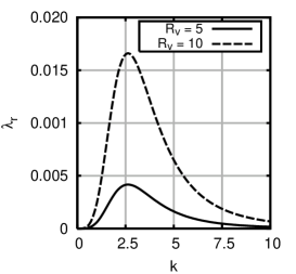
Figure 1: The real part of the growth rate $\lambda_{r}$ as a function of the wave number $k$.

III.4 The case of finite values of vibration number $R_{v}$

In the case of arbitrary values of the vibration parameter $R_{v}$ the boundary value problem (27), (28) was solved numerically. First, the spectrum of eigenvalues was analyzed by the Galerkin method with a basis given by the eigenfunctions gershuni-zhuhovitsky-76 of the problem (27), (28) at $R_{v}=0$, $\lambda\neq 0$. Next, the behavior of the mode with the largest $\lambda_{r}$ was specified by the standard shooting method.stoer-bulirsch-80 It was found that in all the range of the parameters $k$ and $R_{v}>0$ there exists a growth rate with the positive real part $\lambda_{r}>0$: the system turns out to be unstable for any intensity of vibration action. The real part of the growth rate as a function of the wave number (the branch with the maximal $\lambda_{r}$) is plotted in Fig. 1 for different values of vibration parameter $R_{v}$. For any value of the vibration parameter $R_{v}$ the real part of the growth rate $\lambda_{r}$ has a maximum at some value $k_{\ast}$ of the wave number. This critical value $k_{\ast}$ defines the perturbation with the fastest growth rate, which dependence on the vibration parameter is given in Fig. 2. At small values of $R_{v}$ the curve is outgoing from a point with a finite value of $k_{\ast}$. With the growth of vibration intensity the characteristic length scale $k_{\ast}^{-1}$ of hydrodynamic patterns developing as a result of instability of a quasiequilibrium state monotonically decreases.

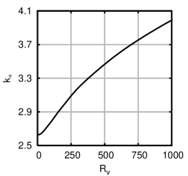
Figure 2: The critical value $k_{\ast}$ of the wave number versus vibration parameter $R_{v}$.

Figure 3 demonstrates the eigenfunction $\hat{\phi}$, which corresponds to the breakdown of the quasiequilibrium and differs from the transversal velocity component by a constant factor. Under vibration action a nonuniformity of the quasiequilibrium distribution of particles leads to generation of the averaged fluid motion, which, in its turn, deforms the initial distribution of particles.

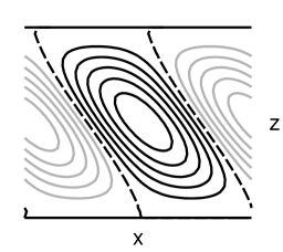
Figure 3: Streamlines of the averaged flow for the perturbation with the fastest growth rate, $R_{v}=10$.

IV Averaged dynamics of a bubbly fluid

IV.1 Basic equations

So far, the disperse phase was assumed to be nondeformable. However, the description of a bubbly fluid in vibration field requires a closer look. The presence of the disperse phase that is able to change its volume under the action of an external periodic field, can drastically influence the pulsation and the averaged dynamics of the system. Next, the case of a monodisperse bubbly fluid is studied and the criterion when compressibility of the disperse phase cannot be neglected is provided. Assuming the concentration $\varphi$ of bubbles to be small, we formulate the equations for the momentum of the liquid carrier phase and the bubbles (2) together with (3), where for our particular consideration $\kappa=0$. An essential modification that has to be taken into account here concerns an additional contribution to the interphase force nigmatulin-91

$${\bf F}_{c}=-\rho\frac{3b}{2r_{d}}{\bf W},$$

where $b$ is the space-averaged radial velocity of bubbles.

Further, assuming that the size of viscous boundary layer $\ell$ is small compared with the time-averaged radius $R$ of a bubble $(\ell\ll R)$, we can neglect the memory forces. yang-leal-91 Indeed, in the frames of the accepted approximation the leading contribution to the pulsation motion is made by the inertia forces [the first and the fourth terms in (3)], whereas for the averaged motion the Stokes force and ${\bf F}_{c}$ are dominant. We suppose the density of the gaseous phase to be much smaller than the density of the fluid and neglect the left-hand side in Eq. (2b), i.e., the force on the bubbles vanishes. The equations defining the kinematics read nigmatulin-91

$${\rm div}\left(1-\varphi\right){\bf U}+{\rm div}\,\varphi{\bf U}_{d} = \frac{3\varphi}{r_{d}}\,b,$$ (35)

$$\frac{d\varphi}{dt}+\varphi\,{\rm div}\,{\bf U}_{d} = \frac{3\varphi}{r_{d}}\,b,$$ (36)

$$\frac{d\rho_{d}}{dt}=-\frac{3}{r_{d}}\,b\rho_{d},\quad\frac{dr_{d}}{dt}=b.$$ (37)

The pressure in the fluid $P$, the pressure in a bubble $P_{g}$ and the velocity of the radial oscillation of a bubble are coupled through the Rayleigh-Plesset equation:nigmatulin-91 ; brennen-95

$$r_{d}\frac{db}{dt}+\frac{3}{2}b^{2}-\frac{1}{4}{\bf W}^{2}=\frac{1}{\rho}\left(P_{g}-\frac{2\sigma}{r_{d}}-P\right).$$ (38)

where $\sigma$ is the surface tension.

According to the procedure laid down in Sec. II, we introduce the time hierarchy, splitting all the fields into the pulsation (depending on the fast time $\tau$) and the averaged parts. The notation and units for the pulsation and averaged components of the velocities, the pressure, and the concentration are the same as used before, in Sec. II. Hereafter, $b$ is the pulsation velocity of radial motion.

IV.2 Pulsation motion

Consider vibration of a cavity entirely filled with a bubbly fluid. The principal assumptions introduced in Sec. II are kept the same: the carrier phase is incompressible, the frequency of vibration is high, but subacoustic, the size of bubbles and the vibration amplitude are small. On the other hand, we impose stronger restrictions for the amplitude $a$ and the frequency $\omega$ of vibration:

$$aL\ll R^{2},\quad\omega\gg\frac{{\rm max}(\nu,\chi,\chi_{d})}{R^{2}},$$ (39)

where $\chi$ and $\chi_{d}$ are the thermal diffusivities of the phases. The second inequality implies that dissipation is unimportant for the pulsation motion, therefore the pressure oscillation of gas obeys an adiabatic law.

Let us now formulate the equations for the pulsation motion. The units for the pulsation velocity and the pressure are kept the same as earlier (see Sec. II.2), as a unit for the velocity of the radial motion we choose $a\omega L/R$. The equation for the pulsation of the concentration $\phi$ splits off and can be treated separately. For this field we obtain

$$\frac{\partial\phi}{\partial\tau}=3\,\frac{aL}{R^{2}}\left(bc-\frac{1}{l}\,{\rm div}\,c{\bf V}\right),\quad l=\frac{L}{R}\gg 1.$$ (40)

As it follows from Eq. (40), the pulsation of the concentration is small compared to the averaged field $c$. Note, that the second term in the right-hand side of Eq. (40) is, generally, much smaller than the first one. However, under certain conditions it becomes non-negligible (see Sec. IV.4).

It is convenient to write down the equations for the remaining pulsation fields in terms of amplitudes. Assuming that all the fields are proportional to $\exp i\tau$, we obtain

$$i(1-c)\hat{\bf V}=-\nabla\hat{q},\quad\hat{\bf V}_{d}=3\hat{\bf V},$$ (41)

$${\rm div}\,(1+2c)\hat{\bf V}=3\,cl^{2}\hat{b},\quad\hat{q}=i\hat{b}(\Omega^{2}-1),$$ (42)

where $\hat{\bf V}$, $\hat{\bf V}_{d}$, $\hat{q}$, $\hat{b}$ are the complex amplitudes of the velocities of the phases, the pressure, and the velocity of the radial motion. Equations (41), (42) contain the following dimensionless parameter:

$$\Omega^{2}=\frac{1}{\rho\omega^{2}R^{2}}\left(3\gamma P_{g}-\frac{2\sigma}{R}\right).$$ (43)

Here, $\Omega$ is the ratio of the eigenfrequency of the volume oscillation of a bubble to the frequency of vibration $\omega$, the parameter $\gamma$ is the adiabatic exponent, and $P_{g}$ is the averaged pressure inside a bubble. Note the known relation between the velocities of the phases in a vibration field:landau-lifshitz-87 the amplitude of oscillation of a bubble in an inviscid fluid is three times as much as that of the fluid.

Equation (42) contains a product of two asymptotic parameters: large $l^{2}$ and small $c$. Depending on the relation between these parameters, different solutions to the pulsation problem is possible. Let us introduce a renormalized concentration $\Phi({\bf r})=l^{2}c\,({\bf r})$. Assuming that this field is finite,caflisch-etal-85 we obtain a Helmholtz equation for a potential $\psi$ of the fluid velocity and the impermeability boundary condition:

$$\nabla^{2}\psi+\frac{3\Phi({\bf r})}{\Omega^{2}-1}\psi = 0,$$ (44)

$$\nabla_{n}\psi|_{\Gamma} = j_{n}.$$ (45)

The amplitudes of the pulsation fields are expressed in terms of the potential $\psi$ as follows:

$$\hat{\bf V}=\nabla\psi,\quad\hat{b}=-\frac{\psi}{\Omega^{2}-1},\quad\hat{q}=-i\psi.$$ (46)

Equation (44) has a form of the stationary Schrödinger equation, in which the role of the scattering potential is played by the averaged concentration field $\Phi({\bf r})$ – the waves are scattered on the nonuniformities of the bubble distribution. The impermeability condition (45) should be imposed on the volume-weighted velocity $(1-c)\hat{\bf V}+c\hat{\bf V}_{d}$, which by virtue of (41) differs from $\hat{\bf V}$ only by a small term $2c\hat{\bf V}$. Note that as the frequency $\Omega$ gets closer to a resonant value $\Omega=1$, the susceptibility of the system to vibration action gets much higher. At the point of the resonance, the performed analysis is no longer valid, because even weak dissipation becomes important and cannot be neglected.

Generally, Eq. (44) can be solved only numerically. However, in the case of a small parameter $\epsilon=\left<\Phi\right>/(\Omega^{2}-1)$, it is possible to obtain the leading part of the solution. Here, $\left<\Phi\right>$ is the value of $\Phi$ averaged all over the volume of the system. Note that the parameter $\epsilon$ can be small for two different reasons: for small concentration $\left<\Phi\right>$ or for small vibration frequencies, $\Omega\gg 1$. Assuming that $z$-axis is aligned along the direction of vibration, we can represent the solution in the form

$$\psi=z-z_{c}+\psi_{1},$$

where the term $z-z_{c}$ corresponds to the solution of (44), (45) for $\Phi({\bf r})=0$ and $\psi_{1}\sim\epsilon$ is defined by a boundary value problem

$$\nabla^{2}\psi_{1} = -\frac{3\Phi({\bf r})}{\Omega^{2}-1}(z-z_{c}),$$ (47)

$$\nabla_{n}\psi_{1}|_{\Gamma} = 0.$$ (48)

Applying the solvability conditions for the problem (47), (48), we find the constant

$$z_{c}=\frac{\int_{V}\Phi z\,dV}{\int_{V}\Phi\,dV},$$ (49)

which has the meaning of the $z$-coordinate of the center of mass for the distribution of bubbles.

Thus, for the case of small $\epsilon$ we obtain

$$\hat{\bf V}={\bf j}+O(\epsilon),\quad\hat{b}=-\frac{z-z_{c}}{\Omega^{2}-1}+O(\epsilon).$$ (50)

IV.3 Averaged motion

We now proceed to the averaging of the governing equations. The equation of the momentum for the averaged motion of the fluid takes the following form:

$$(1-c)\left(\frac{D{\bf u}}{Dt}+\tilde{R}_{v}\overline{{\bf V}\cdot\nabla{\bf V}}\right)-\tilde{R}_{v}\frac{L}{a}\,\overline{\phi\frac{\partial{\bf V}}{\partial\tau}}=-\nabla p+\nabla\cdot(1-c)\varepsilon.$$ (51)

Here, as in Sec. II, $\tilde{R}_{v}=a^{2}\omega^{2}L^{2}/\nu^{2}$ and $\varepsilon$ is the averaged shear rate tensor. From the averaged equation for the bubbles follows

$$\frac{2}{3}\frac{r_{d}^{2}}{L^{2}}\tilde{R}_{v}\,\overline{{\bf V}\cdot\nabla{\bf V}}+\tilde{R}_{v}\,\overline{b{\bf V}}+{\bf u}_{d}-{\bf u}=0,$$

where the first term is small compared to the others. With account of (46), this equation provides a relation between the averaged velocities of the phases:

$${\bf u}_{d}={\bf u}+Q\nabla\psi^{2},\quad Q=\frac{1}{4}\,\frac{\tilde{R}_{v}}{\Omega^{2}-1}.$$ (52)

Here $Q$ is the vibration parameter, which is different to that introduced in Sec. II.

To perform averaging in Eq. (51) we take into account relations (46) and Eq. (40). Retaining only the leading terms, we arrive at the equation

$$\frac{\partial{\bf u}}{\partial t}+{\bf u}\cdot\nabla{\bf u}=-\nabla\Pi+\nabla^{2}{\bf u}+3Q\Phi\nabla\psi^{2}.$$ (53)

While obtaining this equation, we neglect the terms proportional to $c$ and renormalize the pressure; the renormalized variable is denoted by $\Pi$. Variations of the averaged pressure, having in dimensional units the order $\rho b^{2}\sim\rho(a\omega l)^{2}$, are assumed to be much smaller than the averaged pressure $P_{g}$ inside a bubble. This assumption ensures that the averaged radius of the bubbles keeps constant and equals $R$. The absolute value of the averaged pressure becomes insignificant, only its gradient is of importance.

The averaging of the equation for the bubble concentration (36) is straightforward and results in

$$\frac{\partial\Phi}{\partial t}+{\rm div}\,\Phi{\bf u}_{d}=0.$$ (54)

The right-hand side of Eq. (54) vanishes, because the phases of $b$ and ${\bf V}$ are shifted with respect to $\phi$ and $r_{d}$ by a quarter-period. For the same reason, there is no nontrivial contribution to the averaged mass balance equation, which transforms to the incompressibility condition for the fluid

$${\rm div}\,{\bf u}=0.$$ (55)

Equations (52)-(55) together with Eqs. (44), (45) defining the pulsation potential $\psi$, represent a set of equations for the averaged dynamics of a bubbly fluid.

In perfect analogy with the case of nondeformable particles, the averaged motion induced in a boundary layer is negligibly small; the principal effect is caused by the considered mechanism of bulk generation. Thus, at rigid boundaries the conventional no-slip boundary condition for the averaged fluid velocity should be imposed. According to (52), the velocity of the bubbles at the boundaries does not turn to zero. Thus, the boundary conditions for the concentration of bubbles must be prescribed at the inflow boundaries, i.e., where ${\bf n}\cdot{\bf u}_{d}>0$ (${\bf n}$ is the outward normal to a boundary).

Note that the intensity of the averaged flow of the bubbly fluid is significantly (by a factor of $l^{2}$ or $c^{-1}$) higher than for the medium with nondeformable particles (see Sec. II). Contrastingly to the case of nondeformable particles, the latter circumstance enables us to consider the vibration parameter $\tilde{R}_{v}$ to be finite for bubbly fluids. However, for low vibration frequencies, $\Omega\gg 1$, this formalism is no longer valid. To obtain any nontrivial effects, it becomes necessary to consider the vibration parameter $\tilde{R}_{v}$ as asymptotically large, when the vibration mechanisms studied in Sec. II become important and cannot be neglected any more. This situation is of special consideration and is studied in the next section.

IV.4 Low frequency approximation. Transition to a suspension of nondeformable particles

The case of the low (with respect to the frequency of natural oscillation of a bubble) vibration frequency, when $\Omega\gg 1$, should be treated separately. In this particular situation, it is convenient to choose the value $a\omega l/\Omega^{2}$ as a unit for the velocity of the radial motion, the units for the other quantities are kept the same. As a result, the pulsation equations read

$$i(1-c)\hat{\bf V}=-\nabla\hat{q},\quad\hat{\bf V}_{d}=3\hat{\bf V},$$ (56)

$${\rm div}(1+2c)\hat{\bf V}=3\,\Omega_{l}^{2}c\hat{b},\quad\hat{q}=i\hat{b}.$$ (57)

Here $\Omega_{l}=\Omega/l$ is the ratio of the two asymptotic parameters. At large values of $\Omega_{l}$ compressibility of the bubbles becomes insignificant. We note, that a similar result has been found out in Ref. nigmatulin-91, : compressibility of a bubble can be neglected only provided that the dimensionless frequency of the radial oscillation of a bubble is large compared to $l$.

We represent the solution of the pulsation problem (56), (57) in the form of series in the small concentration of bubbles

$$\hat{\bf V}=\hat{\bf V}_{0}+\hat{\bf V}_{1}+\ldots,\quad\hat{q}=\hat{q}_{0}+\hat{q}_{1}+\ldots,\quad\hat{b}=\hat{b}_{0}+\hat{b}_{1}+\ldots,$$

where $\hat{\bf V}_{1}$, $\hat{q}_{1}$, $\hat{b}_{1}\sim c$.

To the zero order the pulsation problem reads

$$i\hat{\bf V}_{0}=-\nabla\hat{q}_{0},\quad{\rm div}\hat{\bf V}_{0} = 0,\quad\hat{q}_{0}=i\hat{b}_{0},$$

$${\bf n}\cdot\hat{{\bf V}}_{0}|_{\Gamma} = j_{n},$$

which admits an obvious solution

$$\hat{{\bf V}}_{0}={\bf j},\quad\hat{b}_{0}=-(z-z_{c}).$$ (58)

In the same way as in Sec. IV.2, the constant $z_{c}$ is obtained from the solvability condition in the next order and takes the form (49).

As in Sec. II, it is necessary to take into account a correction $\hat{{\bf V}}_{1}$ to the pulsation velocity. For further purposes only the vorticity of this field turns out to be important. Thus, from (56) we obtain

$$\nabla\times\hat{{\bf V}}_{1}=\nabla c\times{\bf j}.$$ (59)

Equation (40) for the pulsations of concentration transforms into

$$\frac{\partial\phi}{\partial\tau}=3\frac{a}{L}\left(\Omega_{l}^{-2}bc-{\bf j}\cdot\nabla c\right).$$ (60)

Here, in contrast to Eq. (40), the terms in the right-hand side are of the same order and therefore have to be retained.

Averaging of the equations is performed in the same way as in Secs. II.3, IV.3. As a result we arrive at a set of the averaged equations

$$\frac{\partial{\bf u}}{\partial t}+{\bf u}\cdot\nabla{\bf u} = -\nabla\Pi+\nabla^{2}{\bf u}$$ (61)

$$+{\rm R}_{l}\left({\bf j}{\bf j}\cdot\nabla\Phi+3A\Phi\nabla\hat{b}^{2}\right),$$

$${\rm div}\,{\bf u} = 0,\quad{\bf u}_{d}={\bf u}+{\rm R}_{l}A\nabla\hat{b}^{2},$$ (62)

$$\frac{\partial\Phi}{\partial t} + {\rm div}\,\Phi{\bf u}_{d}=0,$$ (63)

where $A=1/(4\Omega_{l}^{2})$, ${\rm R}_{l}=l^{-2}\tilde{R}_{v}$.

In the limit of low vibration frequency, when $A\to 0$ ($\Omega_{l}\gg 1$), the model reduces to the case of nondeformable bubbles: equations (61)-(63) yield the same model as has been developed in Sec. II [cf. Eqs. (22), (23)]. Indeed, for the case of bubbly fluid, $\delta\ll 1$, and inviscid pulsations, $K\gg 1$, we have $B=1$ [see (79), (80)] and the vibration force $R_{l}\,{\bf j}{\bf j}\cdot\nabla\Phi=R_{v}\,{\bf j}{\bf j}\cdot\nabla c$.

In the opposite limiting case, $A\to\infty$, the compressibility of bubbles becomes of crucial importance; the set of equations transforms to Eqs. (52)-(55). In this case, the solutions of the pulsation problem (58) and (50) coincide (if measured in the same units).

V Evolution of a bubbly fluid in a layer

V.1 Statement of the problem

A rather good understanding of vibration action on the dynamics of a bubbly fluid can be obtained from a one-dimensional consideration. Let us apply Eqs. (52)-(55) to study the vibration dynamics of this medium in an infinite plane layer $-1<z<1$, confined by solid walls, the vibration axis is transversal to the boundaries. The quiescent state with the uniform distribution of bubbles is chosen as the initial one. Symmetry of the equations, boundary conditions, and the initial state enables us to treat the problem in a half of the layer, where the functions $\Phi$ and $\psi$ are even and odd, respectively. The fluid velocity vanishes due to the incompressibility condition (55) and the no-slip boundary conditions at the walls. The concentration and the potential of the pulsation velocity are defined by the following boundary value problem:

$$\psi^{\prime\prime} + \frac{3\Phi}{\Omega^{2}-1}\psi=0,$$ (64)

$$\frac{\partial\Phi}{\partial t} + \left(u_{d}\Phi\right)^{\prime}=0,\quad u_{d}=2Q\psi\psi^{\prime},$$ (65)

$$z = 0:\;\psi=0,\,\Phi^{\prime}=0;\quad z=1:\;\psi^{\prime}=1,$$ (66)

where the prime is used to denote a derivative with respect to $z$.

It is obvious, that the variation of the absolute value of $Q$ results only in changing of the time scale, and without loss of generality, we set further $Q=\pm 1$ (the upper sign corresponds to $\Omega>1$, and the lower one – otherwise). We can also renormalize the initial concentration in such a way that $\Phi(z,t=0)=1$; this leads only to rescaling of the frequency $\Omega$.

We can easily make sure that there exists no quasisteady state, when the fluid and the bubbles are quiescent on average. Indeed, for the quasisteady state it immediately follows from Eqs. (65)

$$\left(\Phi_{0}\psi_{0}\psi_{0}^{\prime}\right)^{\prime}=0,$$ (67)

i.e., $\Phi_{0}={\rm const}/(\psi_{0}\psi_{0}^{\prime})$. As earlier, the subscript “0” stands for indication of the quasisteady state solution.

On the other hand, Eq. (64) then transforms to

$$\psi_{0}^{\prime\prime}+\frac{3\,{\rm const}}{\psi_{0}^{\prime}(\Omega^{2}-1)}=0.$$ (68)

Integrating this equation and taking into account that $\psi_{0}^{\prime}$ is even, we conclude that ${\rm const}=0$ and hence $\Phi_{0}=0$. Note, that this conclusion becomes invalid at the points where $\psi_{0}\psi_{0}^{\prime}=0$.

V.2 Initial stage of evolution

We now turn to investigation of the initial stage of evolution, when an analytical solution can be obtained. We assume, that $\Phi=1+\Phi_{1}(z,t)$, where $|\Phi_{1}|\ll 1$.

Neglecting the small perturbation $\Phi_{1}$ in the Schrödinger Eq. (64), we have

$$\psi_{0}^{\prime\prime}+\frac{3}{\Omega^{2}-1}\psi_{0}=0.$$ (69)

First, consider the case $\Omega>1$, when the vibration frequency is lower than that of the natural oscillation of a bubble. We introduce

$$\alpha^{2}=\frac{3}{\Omega^{2}-1}.$$ (70)

and note that this expression for the wave number $\alpha$ is in agreement with the known disperse relation for waves in a bubbly medium (see, for example, Ref. caflisch-etal-85, ; carstensen-foldy-47, ).

The solution to Eq. (69) with the impermeability condition at the boundaries is as follows

$$\psi=\frac{\sin\alpha z}{\alpha\cos\alpha}$$ (71)

The resonant frequencies correspond to the divergency of (71) and are defined by the expression

$$\Omega_{n}^{2}=1+\frac{12}{\pi^{2}(2n+1)^{2}},\quad n=0,1,\ldots.$$ (72)

Note, that at these frequencies it is necessary to account for dissipation in the pulsation equations.

Taking into account the result (71), we obtain the averaged velocity of the bubbles and the correction to the concentration

$$u_{d}=\frac{\sin 2\alpha z}{\alpha\cos^{2}\alpha},\quad\Phi_{1}=-\frac{2\cos 2\alpha z}{\cos^{2}\alpha}\,t+{\rm const}.$$ (73)

We see that the most rapid decrease of the concentration of bubbles occurs in the vicinities of the points $z_{n}=\pi n/\alpha$, $n\in Z$ – the bubbles tend to leave the nodes of the pulsation pressure; and vice versa, the concentration grows in the antinodes of the pressure. This phenomenon is referred to as the primary Bjerknes effect.bjerknes-06 ; feng-leal-97 However, we stress, that in our case, the bubbles are not just advected by the external nonuniform pulsation field (as in the conventional Bjerknes effect). The presence of the bubbles causes this nonuniformity.

Let us proceed to the opposite range of frequencies, $\Omega<1$. In this case, the frequency of external action is beyond the passband for the bubbly fluid, i.e., the waves decay deep into the layer:

$$\psi=\frac{\sinh\alpha z}{\alpha\cosh\alpha},\quad\alpha^{2}=\frac{3}{1-\Omega^{2}},\quad u_{d}=\frac{\sinh 2\alpha z}{\cosh^{2}\alpha},$$ (74)

Further, for the perturbation of the concentration we find

$$\Phi_{1}=\frac{2\cosh 2\alpha z}{\cosh^{2}\alpha}\,t+{\rm const}.$$ (75)

Thus, the bubbles migrate away from the boundaries of the layer to its center. As it could be expected, at a frequency larger than the resonant frequency of a bubble, the bubbles accumulate in the node of the pressure, at the center of the layer.

V.3 Finite time evolution. Numerical results

At finite times the set of equations (52)-(55), describing one-dimensional dynamics of a bubbly fluid in the layer, was studied numerically. The equation for transfer of the bubbles was integrated by means of the method of characteristics. The equation for the characteristics has an obvious form

$$\frac{dz}{dt}=u_{d}(z,t).$$ (76)

At the characteristics the following relation is fulfilled

$$\frac{d\Phi}{dt}=-u_{d}^{\prime}\Phi.$$ (77)

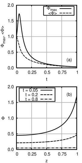
Figure 4: The maximal $\Phi_{max}$ and the averaged $\left<\Phi\right>$ values of concentration as functions of time (a); the concentration profiles at different times, $Q=1,\Omega^{2}=3$ (b).

The fields of the concentration $\Phi$ and potential $\psi$ are defined in the nodes of the uniformly spaced grid; we used up to 2000 grid nodes. In the case when $u_{d}(1)<0$, there appears a front of the concentration $z=z_{s}(t)$ such that $\Phi\neq 0$ only in the domain with $z<z_{s}$. For this particular situation, the grid nodes were interposed only in the domain occupied by the bubbly fluid, i.e., for $z<z_{s}(t)$; in the opposite part of the layer, the equations admit an obvious solution: $\Phi=0$, $\psi=\psi_{0}+z$. At the point $z=z_{s}$ the functions $\psi$, $\psi^{\prime}$ are continuous, so that the value of the constant $\psi_{0}$ is insignificant. In the opposite case, $u_{d}(1)>0$, a part of bubbles settles on the boundaries: the averaged concentration $\left<\Phi\right>=\int_{0}^{1}\Phi\,dz$ decreases with time.

Results of the numerical simulation are presented in Figs. 4-6. If $\Omega>\Omega_{0}=1.489$ [for the uniform distribution of the bubbles, see relation (72)], the bubbles gradually leave the bulk of the layer, settling on the boundaries, Fig. 4. At first, the maximal value $\Phi_{m}$ of the concentration grows and after a while starts to decrease; the averaged concentration $\left<\Phi\right>$ monotonically decreases with time.

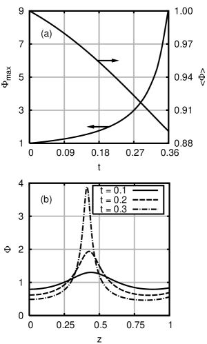
Figure 5: The maximal $\Phi_{max}$ and the averaged $\left<\Phi\right>$ values of concentration as functions of time (a); the concentration profiles at different times, $Q=1,\Omega^{2}=1.25$ (b).

In the case of $\Omega_{1}<\Omega<\Omega_{0}$, the bubbles accumulate in a certain domain inside the layer. The concentration of the bubbles rises abruptly near the point $z_{s}$ and reaches infinite values for a finite time $t=t_{0}$ – there develops a peaking regime. The maximal concentration grows as $(t-t_{0})^{-1}$, i.e., a bubble screen develops. The potential itself remains finite, while its second derivative tends to infinity near the point $z_{s}$. This scenario is demonstrated for $\Omega^{2}=1.25$ in Fig. 5. The averaged concentration of the bubbles decreases with time. As the eigenfrequency $\Omega$ gets closer to $1$, the number of bubble screens increases.

In the case $\Omega<1$, the bubbles accumulate in the center of the layer – a node of the pulsation pressure. Evolution of the maximal concentration, the coordinate $z_{s}$ of a front, i.e., the interface bubbly fluid–pure fluid, and the profiles of the concentration are depicted in Fig. 6. As was mentioned above, the bubbles located near the front possess the maximal velocities [cf. (74)], consequently the concentration grows very fast at the front and does not practically vary in the stagnant core in the center of the layer.

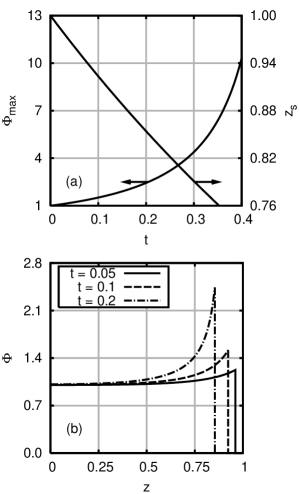
Figure 6: The maximal concentration $\Phi_{max}$ and the coordinate of the front $z_{s}$ as functions of time (a); the concentration profiles at different times, $Q=-1,\Omega^{2}=0.5$ (b).

VI Conclusions

The averaged dynamics of various two-phase systems in a high-frequency vibration field has been theoretically studied. The continuum approach was applied to describe such systems as solid particle suspensions, emulsions, bubbly fluids, when the volume concentration of the disperse phase is small and gravity is insignificant. The dynamics of a monodisperse system was considered by means of the averaging method, when the fast pulsation and slow averaged motion can be treated separately. The vibration dynamics of suspensions of both nondeformable and deformable particles, when the compressibility of the disperse phase becomes important, has been investigated.

An averaged model for nondeformable particles has been obtained. It is shown, that accounting for the Stokes drag and unsteady forces such as the Basset history term, the second memory force and the added mass force in the pulsation motion, is of crucial importance for correct description of the averaged dynamics. The averaged equations have been obtained and simplified in the framework of the single-fluid approximation. It is proven that the particles can be treated as frozen into the averaged fluid flow. As a result the averaged dynamics of a suspension is described by the equations of momentum and mass conservation for the carrier fluid and a transfer equation for the concentration of particles. The action of vibration results in the appearance of a vibration force in the equation of the fluid motion. This force is nonvanishing only for the nonuniform distribution of particles, its direction coincides with the vibration axis. We note, that the developed model is expected to be worth applying to clarify recent experiments on blood flow resistance under vibration action. shin-etal-03

The developed model has been applied to study the behavior of a two-phase medium in an infinite plane layer subjected to transversal vibrations. It is demonstrated that there is a set of possible nonuniform quasiequilibrium distributions of particles, when the averaged flow vanishes but the pulsation velocities do not. The stability of a linear distribution of particles has been investigated. Analytical and numerical analysis manifests that the quasiequilibrium state is unstable for any intensities of vibration. A nonuniformity of particle distributions causes the vibration force that generates the averaged motion in fluid. Because of this flow, the initial distribution of particles is deformed and the state becomes unstable.

As a system with deformable particles, the case of bubbly fluids in vibration field has been analyzed separately. An averaged model accounting for the compressibility of the bubbles has been developed. The pulsations were assumed to be inviscid, and a set of averaged equations has been obtained in the single-fluid approximation. The averaged velocity of bubbles differs from the fluid velocity, this difference is caused by vibration and proportional to its intensity. It is shown that in contrast to the case of nondeformable particles, the impact of vibration on the system with deformable particles is significantly stronger. Even for uniform distribution of particles the vibration force is nonzero.

An intermediate case of low vibration frequencies, when the ratio $\Omega$ of eigenfrequency of radial bubble oscillations to the the frequency of vibration is high, has been considered. A criterion when the compressibility of bubbles can be neglected has been figured out: $\Omega\gg L/R$, where $L$ is the length scale of the flow and $R$ is the time-averaged radius of the bubble. In this case the intermediate model reduces to the model for nondeformable particles. In the opposite limit, $\Omega\ll L/R$, the intermediate model transforms to the discussed model where compressibility of bubbles becomes of crucial importance.

The dynamics of bubbly fluid in an infinite plane layer under the action of transversal vibration has been analyzed. The quiescent state with the uniform distribution of bubbles is chosen as the initial one. It turns out that for $\Omega>1.489$ the bubbles migrate to the boundaries of the layer; for $1<\Omega<1.489$ the bubble screens appear; for $\Omega<1$ bubbles accumulate in the center of the layer. We have demonstrated that the behavior of bubbly fluid is analogous to the primary Bjerknes effect: for $\Omega>1$ the bubbles leave the nodes and accumulate in the antinodes of the pressure wave, while for $\Omega<1$ the bubbles migrate to the nodes. However, in our case, the bubbles are not only advected by the external nonuniform field, as in the conventional Bjerknes effect, but also cause this nonuniformity.

VII Acknowledgments

The research was partially supported by RFBR (Grant No. 04-01-00422) and CRDF (Grant No. PE-009-0), which are gratefully acknowledged. A.S. thanks the German Science Foundation (DFG, SPP 1164); S.S. is thankful to DAAD and Russian Ministry of Education and Science (Russian-German Mikhail Lomonosov Program).

*

Appendix A

Here we analyze relation (21) as a function of the parameters $\delta$, $\kappa$ and $K$. First, we give the expressions for the limiting vibration regimes of viscous ($K\ll 1$) and inviscid ($K\gg 1$) pulsation. Next, we discuss the dependence in the whole range of values of $K$ and outline features for some typical media.

In the limit of viscous pulsation, $K\ll 1$, relation (21) reduces to the following:

$$B_{0}=\frac{(\delta-1)^{2}K^{3}}{9\sqrt{2}}.$$ (78)

Note, in this limit, it is not enough to take into account only the Stokes force, which would result in vanishing $B$ and therefore in no vibration force. Physically, this means that the particles get frozen not only in the averaged flow, but in the pulsation fluid flow as well, and therefore no averaged effects are possible. To account for any nontrivial dynamics one has to retain small (with respect to the Stokes drag) terms due to memory forces, which ensures relative pulsation motion of phases. Another interesting point is that this result does not depend on $\kappa$.

In the opposite limit of inviscid pulsation, $K\gg 1$, the leading contribution to $B$ is made by the added mass force. The result is sensitive solely to the relative density of phases:

$$B_{\infty}=\left(\frac{\delta-1}{1+2\delta}\right)^{2}.$$ (79)

A typical case of a bubbly fluid ($\kappa\ll 1$, $\delta\ll 1$) is governed by

$$B_{b}=\frac{2K^{3}(18\sqrt{2}+9K+3\sqrt{2}K^{2}+K^{3})}{(18\sqrt{2}+18K-K^{3})^{2}+K^{2}(18+3\sqrt{2}K+K^{2})^{2}}.$$ (80)

The result is caused by the Stokes drag, the second memory force, and the added mass force.

For the case of solid particles ($\kappa\to\infty$), the dependence (21) transforms to:

$$B_{s}=\frac{(\delta-1)^{2}\sqrt{2}K^{3}(9+\sqrt{2}K)}{81(\sqrt{2}+K)^{2}+K^{2}[9+\sqrt{2}(1+2\delta)]^{2}},$$ (81)

where the Stokes drag, the Basset and the added mass forces make finite contribution.

To demonstrate the dependence in more general situations, we tabulate (21) as a function of $K$ for different values of $\delta$ and $\kappa$. Typical results are presented in Fig. 7. As it can be shown, the function $B(K)$ is positive for all $K$; it is either monotonic or has a maximum. In the limits of $K\ll 1$ and $K\gg 1$ the results are independent of $\kappa$ and agree with the expressions (78) and (79), respectively. As it can be expected, the effect of different values of $\kappa$ occurs at intermediate values of $K$.

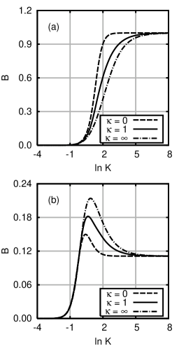
Figure 7: The dependence of $B$ against the parameter $K$ for $\delta=0$ (a) and $\delta=4$ (b).

Figure 7(a) represents the case of bubbly fluids ($\delta\ll 1$); the curve with $\kappa=0$ corresponds to relation (80). The curves go out from the point $B=0$ at $K=0$, start to grow at small $K$ as $K^{3}/(9\sqrt{2})$ [see relation (78)], and monotonically approach the value $B_{\infty}=1$, as follows from (79). For $\delta\leq 1/2$, qualitative form of the curves keep the same as in Fig. 7(a), the value of $B_{\infty}$ changes according to (79).

For $\delta>1/2$ the dependence $B(K)$ is no longer monotonic: there appears a maximum $B_{m}$ at some value $K_{m}$ [see Fig. 7(b)]. The curve with $\kappa\gg 1$ corresponds to solid particles and is described by formula (81); such a curve in Fig. 7(b) is plotted for a suspension “sand in water” ($\delta=4$, $\kappa\gg 1$). We note, that for higher relative densities $\delta$ the dependence $B(K)$ does not change qualitatively. In the limiting case of heavy particles suspended in a gaseous medium (solid particle suspension in air, aerosol), $\delta\gg 1$, the maximum value $B_{m}$ grows and shifts to lower values of $K$; the asymptotic behavior reads $B_{m}\propto\sqrt{\delta}$, $K_{m}\propto 1/\sqrt{\delta}$. At high values of $K$ parameter $B$ gradually approaches the limiting value $B_{\infty}=1/4$.

References

- (1) P. L. Kapitza, “Dynamic stability of a pendulum with an oscillating point of support,” Zh. Eksp. Teor. Fiz. 21, 588 (1951) (in Russian).
- (2) I. I. Blekhman, Vibrational Mechanics: Nonlinear Dynamic Effects, General Approach, Applications (World Scientific, Singapore, 2000).
- (3) P. Evesque and J. Rajchenbach, “Instability in a sand heap,” Phys. Rev. Lett. 62, 44 (1989).
- (4) P. B. Umbanhowar, F. Melo, and H. L. Swiney, “Localized excitations in a vertically vibrated granular layer,” Nature (London) 382, 793 (1996).
- (5) A. Ivanova, V. Kozlov, and P. Evesque, “Patterning of the “liquified” sand surface in a cylinder filled with liquid and subjected to horizontal vibrations,” Europhys. Lett. 35, 159 (1996).
- (6) N. I. Lobov, D. V. Lyubimov, and T. P. Lyubimova, “Behavior of a two-layer liquid-suspension system in a vibration field,” Fluid Dyn. 34, 823 (1998).
- (7) G. Z. Gershuni and D. V. Lyubimov Thermal Vibrational Convection (Wiley, New York, 1998).
- (8) M. Faraday, “On a peculiar class of acoustic figures; and on certain forms assumed by groups of particles upon vibrating elastic surfaces,” Phylos. Trans. R. Soc. London 121, 299 (1831).
- (9) L. Boyadzhiev, “On the movement of a spherical particle in vertically oscillating liquid,” J. Fluid Mech. 53, 545 (1973).
- (10) N. L. Granat, “Motion of a solid body in an oscillating flow of a viscous fluid,” Izv. Akad. Nauk SSSR, OTN Mekhanika i Mashinostroenie 1, 70 (1960) (in Russian).
- (11) V. N. Chelomei, “Paradoxes in the mechanics due to vibrations,” Dok. Akad. Nauk SSSR 270, 62 (1983) (in Russian).
- (12) H. Lamb, Hydrodynamics (Cambridge University Press, Cambridge, 1975).
- (13) B. A. Lugovtsov and V. L. Sennitskii, “The motion of a body in a vibrating liquid,” Dok. Akad. Nauk SSSR 289, 314 (1986) (in Russian).
- (14) D. V. Lyubimov, A. A. Cherepanov, T. P. Lyubimova, and B. Roux, “Vibration influence on the dynamics of a two-phase system in weightlessness conditions,” J. Phys. IV 11, 83 (2001).
- (15) Lord Rayleigh, “On the pressure developed in a liquid during the collapse of a spherical cavity,” Phylos. Mag. 34, 94 (1917).
- (16) M. S. Plesset and A. Prosperetti, “Bubble dynamics and cavitation,” Annu. Rev. Fluid Mech. 9, 145 (1977).
- (17) Z. C. Feng and L. G. Leal, “Nonlinear bubble dynamics,” Annu. Rev. Fluid Mech. 29, 201 (1997).
- (18) V. F. K. Bjerknes, Fields of Force (Columbia University Press, New York, 1906).
- (19) K. Yosioka and Y. Kawasima, “Acoustic radiation pressure on a compressible sphere,” Acustica 5, 167 (1955).
- (20) V. N. Alekseev, “Force produced by the acoustic radiation pressure on a sphere,” Sov. Phys. Acoust. 29, 77 (1983).
- (21) D. Z. Zhang and A. Prosperetti, “Average equations for inviscid disperse 2-phase flow,” J. Fluid Mech. 267, 185 (1994).
- (22) D. Z. Zhang and A. Prosperetti, “Ensemble phase-averaged equations for bubbly flows,” Phys. Fluids 6, 2956 (1994).
- (23) H. F. Bulthuis, A. Prosperetti, and A. S. Sangani, “Particle stress in disperse 2-phase potential flow,” J. Fluid Mech. 294, 1 (1995).
- (24) P. Smereka, “A Vlasov description of the Euler equation,” Nonlinearity 9, 1361-1386 (1996).
- (25) G. Russo and P. Smereka, “Kinetic theory for bubbly flow I: Collisionless case,” SIAM J. Appl. Math. 56, 327-357 (1996).
- (26) V. M. Teshukov and S. L. Gavrilyuk, “Kinetic model for the motion of compressible bubbles in a perfect fluid,” Eur. J. Mechanics B: Fluids 21, 469 (2002).
- (27) L. van Wijngaarden, “One-dimensional flow of liquids containing small gas bubbles,” Annu. Rev. Fluid Mech. 4, 369 (1972).
- (28) R. I. Nigmatulin, Dynamics of Multiphase Media (Hemisphere, New York, 1991).
- (29) R. F. Ganiev and V. F. Lapchinsky, Problems of Mechanics in Cosmic Technology (Mashinostroenie, Moscow, 1978), in Russian.
- (30) M. R. Maxey and J. J. Riley, “Equation of motion for a small rigid sphere in a non-uniform flow,” Phys. Fluids 26, 883 (1983).
- (31) S.-M. Yang and L. G. Leal, “A note on memory-integral contributions to the force on an accelerating spherical drop at low Reynolds number,” Phys. Fluids A 3, 1822 (1991).
- (32) R. Clift, J. R. Grace, and M. E. Weber Bubbles, Drops, and Particles (Academic Press, New York, 1978).
- (33) S. Kim and S. J. Karrila Microhydrodynamics: Principles and Selected Applications (Butterworth-Heinemann, Boston, 1991).
- (34) A. H. Nayfeh, Introduction to Perturbation Techniques (Wiley, New York, 1981).
- (35) H. Schlichting, Boundary Layer Theory (McGraw-Hill, New York, 1968).
- (36) G. Z. Gershuni and E. M. Zhukhovitsky, Convective Stability of Incompressible Fluid (Keter, Jerusalem, 1976).
- (37) J. Stoer and R. Bulirsch, Introduction to Numerical Analysis (Springer, New York, 1980).
- (38) C. E. Brennen, Cavitation and Bubble Dynamics (Oxford University Press, Oxford, 1995).
- (39) L. D. Landau and E. M. Lifshitz, Fluid Mechanics (Pergamon Press, Oxford, 1987).
- (40) R. E. Caflisch, M. J. Miksis, G. C. Papanicolaou, and L. Ting, “Effective equations for wave propagation in bubbly flow,” J. Fluid Mech. 153, 259 (1985).
- (41) E. L. Carstensen and L. L. Foldy, “Propagation of sound through a liquid containing bubbles,” J. Acoust. Soc. Am. 19, 481 (1947).
- (42) S. Shin, Y. Ku, J.-S. Suh, S.-Y. Moon, and J.-Y. Jang, “Characteristics of blood flow under transverse vibration: red blood cell suspension in dextran-40,” Ann. Biomedical Engineering 31, 1077 (2003).