Capture of particles of dust by convective flow

Abstract

Interaction of particles of dust with vortex convective flows is under theoretical consideration. It is assumed that the volume fraction of solid phase is small, variations of density due to nonuniform distribution of particles and those caused by temperature nonisothermality of medium are comparable. Equations for the description of thermal buoyancy convection of a dusty medium are developed in the framework of the generalized Boussinesq approximation taking into account finite velocity of particle sedimentation. The capture of a cloud of dust particles by a vortex convective flow is considered, general criterion for the formation of such a cloud is obtained. The peculiarities of a steady state in the form of a dust cloud and backward influence of the solid phase on the carrier flow are studied in detail for a vertical layer heated from the sidewalls. It is shown that in the case, when this backward influence is essential, a hysteresis behavior is possible. The stability analysis of the steady state is performed. It turns out that there is a narrow range of governing parameters, in which such a steady state is stable.

I Introduction

Disperse systems, such as clouds of small particles suspended in liquid or gas are widespread in natural environment as well as in various fields of human activity. Due to admixture, such systems demonstrate intriguing physical effects, which cannot occur in homogeneous media. Understanding of the mechanisms governing the behavior of particles in fluid flows is of crucial importance both for fundamental studies and practical applications.

Advection of particles in fluid flows is currently investigated in several disciplines. In chemistry (see, for example, Refs. williams-85, ; peters-00, ), this problem is essential in lowering fuel consumption during combustion of liquid fuels. In biology, recent developments have put forth a number of fascinating problems concerning transport of microorganisms in aqueous medium.koch-meinhardt-94 ; abraham-98 ; delgiorgio-duarte-02 A typical example are algae, transported by ocean flows. These algae contribute essentially to the absorption of ${\rm CO}_{2}$ in oceans, which is closely related to the problem of climate change. In rapidly developing microfluidics, advection of particles has been the focus of close attention due to a need of finding effective mechanisms of particle mixing.ottino-89 In fluid mechanics light-scattering particles of dust are widely used for visualization of flows. Besides, it is also important to know how particles influence the flow. Investigation of a spread of fine-dispersed impurities in the atmosphere and oceans is tightly related to the problem of environmental protection. These numerous applications have motivated the unflagging interest in the fundamental problems of particle advection in fluids.

The behavior of a small single particle in isothermal fluid flows has been the subject of a great deal of study (see, for example, the monograph soo-67 and the reviews marble-70 ; maxey-90 ). In particular, the equation of motion for a small single particle in a nonuniform unsteady flow was discussed by Maxey and Riley.maxey-riley-83 However, the fact that this equation takes into account the integral Basset force essentially complicates its solution. Therefore in most cases the problem has been solved in terms of asymptotic theoretical models. Stommel stommel-49 studied sedimentation of particles in a cellular fluid flow in terms of weak inertia approximation. To our knowledge this was the first paper that developed a simple description of capture of small solid particles by a fluid flow. It was shown, that when the ascending flow is rather intensive, some particles are involved in a vortex motion and remain suspended. Recently, capture of particles has been observed in a cellular convective flow.simon-pomeau-91 Qualitatively similar behavior is shown by granular media in the ascending air flow under gravity: at a certain velocity of air flow the granular matter is liquidized.anderson-etal-95 The problem of sedimentation of small heavy particles has been generalized for the case of a random flow (see Ref. pasquero-etal-03, and references therein). However, a backward effect of the particles on a fluid flow was not considered. A number of theoretical and experimental studies are devoted to the problem of particle accumulation in fluid flows – the effect, which is essential due to a difference in the inertial properties of the phases when gravity is insignificant.tio-etal-93 ; druzhinin-95-phf ; druzhinin-95-jfm ; schwabe-frank-99 The situation, when both gravity and inertia contribute to the particle dynamics, has been studied in papers.maxey-corrsin-86 ; maxey-87 ; davila-hunt-01 The authors of papers thomas-92 ; druzhinin-ostrovsky-94 ; yanna-etal-97 ; mordant-pinton-00 ; armenio-fiorotto-01 ; candelier-etal-04 have investigated the influence of the Basset history force on the particle motion.

Another problem that has been intensively studied for many years is the stability of laminar isothermal flows carrying small solid particles. First papers saffman-62 ; michael-64 ; liu-65 were devoted to the stability of the particulate Poiseuille flow. This problem has been generalized in the series of papers.isakov-rudyak-95 ; rudyak-isakov-bord-97 The stability of the Couette flow was considered in Ref. drew-75, . A general result of these investigations is that stability of a dusty flow qualitatively depends on the size of particles: relatively small particles destabilize the flow, whereas the particles of a larger size make the flow more stable. The relaxation time of small particles is short, therefore such particles move actually with the velocity of the fluid. The presence of particles results in renormalization of the media density. A larger efficient density is equivalent to a higher fluid velocity, which leads to destabilization. On the contrary, the relaxation time of large particles is long. Such particles are too inert to respond to rapid velocity variations of the carrying fluid and hence, large particles damp the fluid velocity perturbations.

The collective behavior of particles in laminar nonisothermal flows is much less studied. Moreover, the problem of interaction of the particles with convective flows is not completely understood yet. The exceptions are the works, concerning the influence of settling particles on the stability of convective flows.dementyev-96 ; dementyev-00 ; lyubimov-etal-98

It is known, that particles of dust are widely used for visualization of flows in the experiments on thermal buoyancy convection. It is conventionally assumed that, if the mass concentration of particles is small, their backward influence on the convective flow is negligible. However, this is not always true. The point is that buoyancy convective flow itself is caused by small variations of density related to nonisothermality of a medium. If density variations due to nonuniformity of the particle distribution are of the same order of magnitude as those due to nonisothermality, one should no longer ignore the influence of particles on the flow. For small particle concentration this effect is intuitively believed to be pronounced if the density of particles and the density of the carrier fluid differ enough. A typical example is solid particles suspended in a gaseous medium. However, we argue below that the effect is essential in more general case, when the densities of phases are different, but of the same order (for example, in liquids laden with small solid particles). Under gravity such particles tend to settle on the bottom of a container. Two mechanisms hinder particles from settling down: the Brownian motion of particles leading to their diffusion in a carrier fluid and the entrapment of particles by vortex fluid flows. The first mechanism operates also in a quiescent medium and leads to the Boltzmann distribution of particles over a height. However, for particle sizes commonly used for flow visualization, an effective diffusion coefficient is so small that in the equilibrium state the particles are practically absent in most part of the volume. The second mechanism, which operates only if the maximal velocity of ascending flows exceeds the sedimentation velocity, is much more efficient. Investigation of the capture effect and a backward influence of the particles on a flow is important not only for visualization problems but also for more fundamental aspects of environmental problems.

The mechanism of particle capture discussed above is related to nonuniformity of the particle distribution over the volume. Even if the initial distribution of particles is uniform, this nonuniformity arises by itself due to the particle sedimentation in the regions, where the flow is either descending or has small vertical velocities. If the vertical dimension of the container is large, the particle distribution in the most part of the container is nearly uniform for a long time. However, even in this case the particles can influence the flow, because their velocity differs from the velocity of the fluid due to sedimentation. Thus, the particles can transfer the perturbations of temperature and vorticity and affect stability of a convective flow.dementyev-96 ; dementyev-00

In the present paper, we study the capture of dust particles by convective flows. Particularly, a backward effect of particles on the fluid flow is investigated in details. In Sec. II, an appropriate theoretical model is developed as a generalization of the Boussinesq approximation to a convective flow in a dusty medium. In Sec. III, the obtained equations are used to make a general interpretation of the problem and to prove that the entrapped particles form a cloud of dust. Section IV is devoted to consideration of a dusty medium in an infinite vertical layer. The existence of a steady state solution with particle distribution in the form a dust cloud is proved, and the stability of this state is investigated.

II Theoretical model of thermal buoyancy convection in a dusty medium

II.1 Governing equations and basic assumptions

Consider the behavior of small solid particles, suspended in a nonisothermal fluid (liquid or gas) under gravity. On one hand, all particles are assumed to be monodisperse spheres of a radius $r_{p}$, which is large enough to neglect particle diffusion. On the other hand, this size is supposed to be much smaller than the characteristic length scale $L$ of the flow. On a scale much greater than $r_{p}$ the particles are regarded as a continuous medium with the volume fraction $\varphi=4/3\pi r_{p}^{3}n$ (the volume fraction of the fluid phase $\mu=1-\varphi$), where $n$ is the the number of particles per unit volume of the medium. Since the actual volume concentration $n$ is proportional to $\varphi$ and differs from the latter by a constant factor, in the following for the sake of simplicity $\varphi$ will be called concentration.

We suppose that the volume concentration of particles is small, so we can neglect interparticle interactions and interactions between the particles and walls of a container. It is also assumed that the carrier phase is incompressible and the solid particles can neither deform nor combine into agglomerates. Moreover, the density of a solid phase is considered to be constant. The latter assumption implies that we neglect thermal expansion of the solid phase, which is perfectly valid in the dilute limit. After averaging over space the equations for mass, momentum and energy balance of both phases are written as follows: soo-67 ; marble-70 ; nigmatulin-91

$$\frac{\partial\left(\mu\rho\right)}{\partial t}+{\rm div}\left(\mu\rho{\bf u}\right) = 0,$$ (1a)

$$\frac{\partial\varphi}{\partial t}+{\rm div}\left(\varphi{\bf u}_{p}\right) = 0,$$ (1b)

$$\mu\rho\frac{D\bf u}{Dt} = -\nabla p+\nabla\cdot\left(\mu{\bf\varepsilon}\right)-\mu\rho{\rm Ga}\,{\bf e}_{z}-\varphi{\bf F},$$ (2a)

$$\delta\,\frac{d{\bf u}_{p}}{dt} = -\delta\,{\rm Ga}{\bf e}_{z}+{\bf F},$$ (2b)

$$\mu\rho\frac{DT}{Dt} = \frac{1}{\rm Pr}{\rm div}\left(\mu\nabla T\right)+\frac{3}{\rm Pr}\frac{L^{2}}{r_{p}^{2}}\varphi\left(T_{p}-T\right),$$ (3a)

$$\delta\,{\rm B}\frac{dT_{p}}{dt} = -\frac{3}{\rm Pr}\frac{L^{2}}{r_{p}^{2}}\left(T_{p}-T\right),$$ (3b)

where ${\bf u}$ and ${\bf u}_{p}$, $T$ and $T_{p}$, are the velocities and the temperatures of phases, $p$ and $\rho$ are the pressure and the density of fluid, respectively (hereafter, the subscript $``p"$ stands for the particle phase), ${\bf e}_{z}$ is the unit vector of the axis $z$, directed against gravity; the shear rate tensor $\varepsilon_{ij}=\nabla_{i}u_{j}+\nabla_{j}u_{i}$. The dimensionless variables have been introduced using the following units: the reference density of fluid $\rho_{0}$ for the densities of phases, the reference temperature difference $\theta$ for the temperatures, $L$ for the coordinates, $L^{2}/\nu$ for the time, $\nu/L$ for the velocities, $\rho_{0}\nu^{2}/L^{2}$ for the pressure, where $\eta$ is the viscosity of fluid and $\nu=\eta/\rho_{0}$.

Equations (1)-(3) involve the following dimensionless parameters: the Galilei number ${\rm Ga}=gL^{3}/\nu^{2}$, the Prandtl number ${\rm Pr}=\eta c/\kappa$, the ratio of densities of phases $\delta=\rho_{p}/\rho_{0}$, the ratio of the specific heats of phases at constant pressure ${\rm B}=c_{p}/c$ and the ratio of characteristic particle size to the flow length scale $r_{p}/L$, where $\kappa$ is the thermal conductivity of fluid. We make a note of the distinction between the two Lagrangian derivatives $D/Dt=\partial/\partial t+{\bf u}\cdot\nabla$ and $d/dt=\partial/\partial t+{\bf u}_{p}\cdot\nabla$, which are used to denote the time derivative associated with the motion of the fluid element and the element of a solid phase, respectively.

In the interphase interaction term, ${\bf F}$ has the meaning of the force exerted by an unsteady nonuniform fluid on the solid particle. This force can be written as maxey-riley-83 ; nigmatulin-91

$${\bf F} = \rho\left(\frac{D\bf u}{Dt}+{\rm Ga}{\bf e}_{z}\right)-\frac{9}{2}\frac{L^{2}}{r_{p}^{2}}{\bf W}$$ (4)

$$-\frac{9}{2}\frac{L}{r_{p}}\sqrt{\frac{\rho}{\pi}}\int\limits_{0}^{t}\frac{d{\bf W}(\tau)}{d\tau}\frac{d\tau}{\sqrt{t-\tau}}-\frac{1}{2}\rho\frac{d{\bf W}}{dt},$$

where the relative velocity of phases ${\bf W}={\bf u}_{p}-{\bf u}$ is introduced. The first two terms in (4), correspond to contributions to the force exerted on the particle by undisturbed fluid flow due to gravity and pressure gradient. In the approximation of undisturbed flow these terms coincide with the Archemedian force. Generally, the particle during its motion, disturbs the flow, the effect being taken into account by the next three terms in (4): the Stokes viscous drag, the Basset history force, caused by unsteadiness of a viscous boundary layer around a particle, and the added mass force, allowing for the inertia of the surrounding fluid.

We do not consider the effects that can be initiated by rotation of particles. Particularly, the Magnus force is not taken into account in (4). This assumption holds only in the case when the particle response time $2{r_{p}^{2}}\delta/(9\nu)$ is much less than the characteristic hydrodynamic time scale $L^{2}/\nu$. Therefore the Stokes number, corresponding to a ratio of these time scales, is assumed to be small:

$${\rm St}=\frac{2}{9}\frac{r_{p}^{2}}{L^{2}}\delta\ll 1.$$

However, we assume the parameter $\delta$ to be finite and do not restrict our theory to the limiting case of dusty media ($\delta\gg 1$), cf. Refs druzhinin-95-phf, ; druzhinin-95-jfm, . Further, we do not explicitly take into account Einstein’s correction term to the viscosity of fluid due to solid admixture, which is inessential in the dilute limit.

The equation of state used here is typical for thermal buoyancy convection. We consider weak convection, when the variations of density due to nonisothermality of a fluid are small. Assuming that the fluid density is a function of only temperature $\rho=\rho(T)$, we expand it into a Taylor series near its reference value $\rho_{0}$ at the temperature value $T_{0}$ and restrict ourselves to a linear approximation

$$\rho=1-\beta\theta T,\qquad\beta\theta\ll 1,$$

where temperature $T$ is measured from the value $T_{0}$, $\beta$ is the thermal expansion coefficient.

II.2 Single-fluid approximation

Let us consider a fluid laden with small solid particles and prove that the initial two-phase theoretical model (1)-(4) can be simplified. We assume that the mass concentration of particles $\delta\varphi$ is comparable with the relative variations of the fluid density due to nonisothermality. Bearing in mind that the particle concentration $\varphi$, the nonisothermality $\beta\theta$, and the relative size of particles $r_{p}/L$ are small we retain only the leading terms in the momentum equations (2). As a result we conclude that in the basic state the pressure distribution is hydrostatic, and obtain a relation between the velocities of phases:

$$\nabla p+{\rm Ga}{\bf e}_{z} = 0,$$ (5)

$${\bf u}_{p}={\bf u}-{\rm S}{\bf e}_{z},\qquad{\rm S} = \frac{2}{9}\frac{r_{p}^{2}}{L^{2}}(\delta-1){\rm Ga},$$ (6)

where $\rm S$ is the dimensionless sedimentation velocity. Equation (6) indicates that in the accepted approximation the particle velocity equals the velocity of the fluid plus the constant sedimentation velocity.

Taking into account (6), we obtain in the next order the momentum equation of the fluid

$$\frac{\partial{\bf u}}{\partial t}+{\bf u}\cdot\nabla{\bf u}=-\nabla p^{\prime}+{\nabla}^{2}{\bf u}+\left[\beta\theta\,T-(\delta-1)\varphi\right]{\rm Ga}{\bf e}_{z},$$ (7)

where $p^{\prime}$ is the convective addition to the hydrostatic pressure. Following the idea of the Boussinesq approximation we can state that at large values of the Galilei number and small density inhomogeneities the density of the medium will be constant everywhere except for the buoyancy force, where these small density variations are multiplied by ${\rm Ga}$. So, we introduce the thermal Grashof number ${\rm Gr}=\beta\theta{\rm Ga}$ and its concentration analog ${\rm Gc}=(\delta-1)\varphi_{0}{\rm Ga}$, where $\varphi_{0}$ is the characteristic value of the particle concentration.

From the energy balance equation (3b) we obtain in the leading order: $T_{p}=T$. We restrict our consideration to this approximation. This implies that for small particles the time to equilibrate the phase temperature is much less than the viscous hydrodynamic time scale. The energy equation for the fluid phase is then obtained from Eqs. (3).

Taking into account the mass balance equations for fluid and particles (1) we arrive at a complete set of equations describing thermal buoyancy convection in a nonisothermal fluid laden with particles:

$$\frac{\partial{\bf u}}{\partial t}+{\bf u}\cdot\nabla{\bf u} = -\nabla p+{\nabla}^{2}{\bf u}+\left({\rm Gr}\,T-{\rm Gc}\varphi\right){\bf e}_{z},$$ (8)

$$\frac{\partial T}{\partial t}+{\bf u}\cdot\nabla T = \frac{1}{{\rm Pr}}{\nabla}^{2}T,$$ (9)

$$\frac{\partial\varphi}{\partial t}+{\bf u}_{p}\cdot\nabla\varphi = 0,$$ (10)

$${\rm div}\,{\bf u} = 0,\quad{\bf u}_{p}={\bf u}-{\rm S}{\bf e}_{z},$$ (11)

where the prime for $p$ is omitted, and the concentration is normalized by $\varphi_{0}$.

The set of equations (8)-(11) is reminiscent of equations for thermosolutal convection. However, there are two essential differences: first, we have neglected the diffusion of particles, second, we have taken into account the finite sedimentation velocity. The developed model is quite general and can be applied to dusty media, aerosols, liquids laden with small solid particles, and biological species in aqueous media.

III Capture of dust particles. General consideration

Consider the behavior of a dusty medium in a closed cavity of an arbitrary shape heated from the sidewalls. It is assumed that at the initial time the dust is uniformly distributed all over the volume and at a later time no new particles enter the cavity but the existing particles may settle to the bottom. We also assume that the particles that have settled on the bottom are not carried back into the flow, but stick to the bottom. The question arises as to whether all particles should eventually settle on the bottom or there may occur a situation when some particles will be entrapped by the flow and stay in a suspended state for infinitely long time.

Obviously, in the absence of heating (${\rm Gr}=0$) and any initial perturbations, all particles will eventually sink down on the bottom for a time of order $1/{\rm S}$, which corresponds to the following solution of the equations (8)-(11):

$${\bf u} = 0,$$

$$T = 0,$$

$$\varphi = \begin{cases}0,&z>Z(t)\\ 1,&z<Z(t)\end{cases}$$

where $Z(t)={\rm const}-{\rm S}\,t$. So, initial distribution of particles ensures sedimentation without distortion of the interface between a pure fluid and suspension.

In order to simplify further argumentation, we will measure $z$ from the lowest point of the cavity. It can be understood through insight that inducing of initial perturbations of concentration and velocity does not change the situation: finally all perturbations will be damped and all the particles will settle on the bottom. To demonstrate this let us consider the evolution of the total energy of the system $E$:

$$E=\int_{\Omega}\left(\frac{u^{2}}{2}+{\rm Gc}\,\varphi z\right)d\Omega.$$ (12)

Using (8)-(11) we obtain for the rate of the energy change

$$\frac{dE}{dt}=-\int_{\Omega}{\left(\nabla\times\,{\bf u}\right)}^{2}d\Omega+\oint_{F}\varphi z\,{\bf e}_{z}\cdot{\bf n}\,dF,$$ (13)

where $F$ is the surface bounding the volume $\Omega$, ${\bf n}$ is the external vector normal to $F$. To obtain Eq. (13) the no slip conditions for fluid velocity are assumed: ${\bf u}|_{F}=0$. Since at all time moments $t>0$ the value $\varphi$ differs from zero only on such areas of the boundary surface where ${\bf e}_{z}\cdot{\bf n}<0$ (i.e. at the bottom of a cavity), the right-hand side of (13) is always nonpositive. Moreover it can be equal to zero only in the case of a quiescent fluid in the absence of the particles at the walls. This proves that the energy $E$ can only decrease. On the other hand, as can be seen from (12), $E\geq 0$, i.e. it is bounded from below. Hence, the final state is that, at which the right-hand side in (13) turns to zero, i.e. when the fluid becomes completely free of the particles and all fluid flows cease.

The situation radically changes if there is a permanent external source that makes fluid move. In the present work, the source of this kind is side heating of the wall, generating a vortex convective flow in a cavity. Naturally, in this case, the areas near the walls will finally be free of particles. Indeed, as it follows from Eq. (10)

$$\frac{d}{dt}\int_{\Omega}\varphi\,d\Omega=-\int_{\Omega}{\bf u}_{p}\cdot\nabla\varphi\,d\Omega={\rm S}\oint_{F}\varphi\,{\bf e}_{z}\cdot{\bf n}\,dF\leq 0.$$ (14)

The total amount of the dust in the cavity decreases until $\varphi$ turns to zero everywhere near the boundaries. It does not mean, however, that the bulk of the fluid will be completely free of particles. If in some part of the cavity the velocity of the ascending fluid $u_{a}$ exceeds the sedimentation velocity ${\rm S}$, we can expect the capture of the particles. The condition

$$u_{a}>{\rm S}$$ (15)

is the necessary condition for capture but it is not a sufficient one. Indeed, we can easily imagine the flow pattern with the streamlines of particles shown in Fig. 1(a): despite the existence of regions with ascending motion of particles, all streamlines end at the lower boundary.

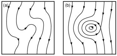
Figure 1: Streamlines of the particle flow in the absence (a) and in the case (b) of particle capture.

On the other hand, we can specify a sufficient condition for capture, which is probably not necessary. Let us assume that there is the line, at which the horizontal component of the the fluid velocity vanishes. If on this line there is a point where $u_{a}={\rm S}$ then such a point is a singular point for the vector field ${\bf u}_{p}$. Furthermore, owing to (11) we have

$${\rm div}\,{\bf u}_{p}=0,$$

and therefore the vector field ${\bf u}_{p}$ is free of sources or sinks. In this case only two types of structurally stable fixed points are possible: center or saddle. In the case of the center point, there are closed orbits, i.e. some particles are entrapped by a vortex and stay inside for infinitely long time. The existence of the saddle point together with the boundary conditions for ${\bf u}_{p}$ necessary implies the existence of the closed separatrix loop and the center point, as it is schematically presented in Fig. 1(b). The separatrix loop forms the boundary of the captured cloud of particles.

To demonstrate how formation of a cloud of dust occurs, we have numerically integrated Eqs. (8)-(11) for a partial case of the square cavity, heated from the right side. The quiescent state with uniform distribution of particles was chosen as the initial one. The values of governing parameters correspond to the single-vortex flow, satisfying the condition (15). This complementary example is in agreement with the results of general consideration. During evolution (see Fig. 2), a part of particles is gradually leaving the flow, whereas other particles stay suspended. As a result of this transient process, the system evolves to the steady state with a distribution of particles in the form of a cloud.

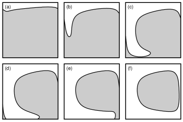
Figure 2: Evolution of particle concentration $\varphi$ to the steady state at ${\rm Gr}=10~{}000$, ${\rm S}=5$, ${\rm Gc}=0$. The times for the states of $\varphi$ are: (a) $t=0.02$, (b) $t=0.04$, (c) $t=0.07$, (d) $t=0.09$, (e) $t=0.14$, (f) $t=0.40$. The regions of pure liquid and particle suspension are shown in white and grey respectively.

The theory above describes the case of no particle inertia. In general, the trajectory of a captured particle is no longer a closed orbit. Due to inertia the center fixed point [see Fig. 1(b)] transforms to a focus, which is unstable for heavy particles.maxey-90 In the vicinity of the focus, captured particles of dust are repelled by this fixed point and move along spirals. Nonetheless, for small particles this effect is weak. The addition to the velocity of particle due to purely inertial drift ${\bf u}_{p}^{in}$ is given druzhinin-95-phf ; druzhinin-95-jfm by the term ${\rm St}\,{D\bf u}/{Dt}$. Since the intensity of thermal convection is governed by the thermal Grashof number, we can estimate ${\bf u}_{p}^{in}\sim{\rm St}\,{\rm Gr}$. For fine particles of dust with $r_{p}\sim 10^{-4}~{}\rm cm$ suspended in air on laboratory length scales $L\sim 1~{}\rm cm$ at moderate intensity of thermal convection we obtain the inertial time scale $\tau_{in}\sim 10^{3}~{}\rm s$ (${\rm St}\sim 10^{-5}$, ${\rm Gr}\sim 10^{3}$).

Recall, that we have also neglected the diffusion of the particles, which means that our consideration concerns the time scales less than the diffusion time scale $t_{d}$. However, this restriction is practically of no significance. Indeed, according to the Einstein formula, the diffusion coefficient of the spherical particles $D=kT/(6\pi\eta r_{p})$ (here $T$ is the absolute temperature, $k$ is the Boltzmann constant). As before, for the fine particles of dust in air at room temperature we obtain $D\sim 10^{-7}~{}\rm{cm^{2}/s}$, which for the laboratory length scales corresponds to the diffusion time scale $t_{d}\sim 10^{7}~{}\rm s$ ($r_{p}\sim 10^{-4}~{}\rm cm$, $L\sim 1~{}\rm cm$).

Thus, despite the fact that existence of a state with a cloud of dust is in general not everlasting due to particle inertia and particle diffusion, it exists long enough to be important.

IV Cloud of dust in a vertical layer

IV.1 Basic steady state

A rather complete understanding of the mechanisms responsible for formation of a cloud of dust and its backward influence on the flow hydrodynamics can be obtained from a model problem. Let a dusty medium fill the infinite vertical layer $-1<x<1$, the boundaries of which are kept at constant, but different temperatures: $T=-1$ at $x=-1$ and $T=1$ at $x=1$. We assume that initial distribution of particles is uniform and look for a steady state solution, in which the velocity has only vertical component $u_{0}$ and all fields except for the pressure are independent of the vertical coordinate $z$. Then, the set of equations (8)-(11) takes the form:

$$u_{0}^{\prime\prime}+{\rm Gr}\,T_{0}-{\rm Gc}\varphi_{0} = c,$$ (16)

$$T_{0}^{\prime\prime} = 0,$$ (17)

where the prime stands for differentiation with respect to $x$, the subscript $``0"$ is used to indicate the steady state solution, $c=\partial p/\partial z=\rm{const}$. Equations (16), (17) should be supplemented with the boundary conditions for the fluid velocity and the temperature:

$$x=\pm 1:\quad u_{0}=0,\quad T_{0}=\pm 1.\\$$ (18)

In the case of the infinite layer we should also specify integral conditions. We prescribe no-flux for fluid and particles, which mean that the flow is closed at the infinity and no new particles enter the system:

$$\int\limits_{-1}^{1}u_{0}\,dx=0,\quad\int\limits_{-1}^{1}\varphi_{0}\,u_{p\,0}\,dx=0,$$ (19)

where $u_{p\,0}=u_{0}-{\rm S}$.

According to (17), (18), the temperature distribution does not depend on the fluid and particle motions and can be obtained directly

$$T_{0}=x.$$ (20)

Let us analyze velocity profiles of the fluid and solid phase. We start the discussion with the simplest case $\rm Gc=0$, when the particles do not influence the fluid motion. In this case, the velocity profile of the fluid is exactly the same as in the well-known problem on a convective flow of pure fluid in a vertical layer heated from the sidewalls:gershuni-zhuhovitsky-76

$$u_{0}=\frac{{\rm Gr}}{6}\,x\left(1-x^{2}\right).$$ (21)

The particles occupy the region of the layer between $x_{1}$ and $x_{2}$. Within this interval $\varphi_{0}=1$, whereas in the near-wall regions $\varphi_{0}=0$.

The point $x_{2}$ is the point at which the velocity of particle sedimentation coincides with the velocity of the ascending fluid flow

$$x=x_{2}:\quad u_{0}={\rm S}.$$ (22)

According to (21), it is determined by the largest root of the cubic equation

$${\rm Gr}\,x_{2}\left(1-x_{2}^{2}\right)=6{\rm S}.$$ (23)

The point $x_{1}$ is determined by the zero-flux condition (19) for particles. It is convenient to rewrite the equation for $x_{1}$ in terms of semi-width of the cloud $d=(x_{2}-x_{1})/2$ (hereafter, just width). Thus, we obtain for $d$

$$d=x_{2}-\sqrt{\frac{1-x_{2}^{2}}{2}}.$$ (24)

As evident from Eq. (23) and the second condition in (19), the parameter ${\rm S}$ is not independent; the width of the cloud is determined by the ratio ${\rm Gr}_{0}={\rm Gr/S}$, moreover, the cloud exists only if ${\rm Gr}_{0}>9\sqrt{3}$. With the growth of ${\rm Gr}_{0}$ the width of the cloud monotonically increases and tends to $1$ as ${\rm Gr}_{0}\to\infty$ (see Fig. 3).

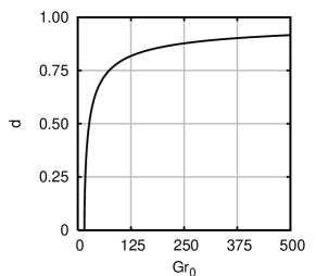
Figure 3: The width of a dust cloud $d$ versus ${\rm Gr}_{0}$ at ${\rm Gc}=0$.

At nonzero values of ${\rm Gc}$ the particles exercise an influence on the fluid flow, and the dependence of the characteristics of the cloud on the parameters becomes more complex. In this case the basic state is governed by ${\rm Gr}_{0}$ and a renormalized concentration parameter ${\rm Gc}_{0}={\rm Gc/S}$. In the presence of a particle cloud the flow region splits into three zones: 1) $-1<x<x_{1}$, 2) $x_{1}<x<x_{2}$, 3) $x_{2}<x<1$. In each of these zones the velocity profile is described by third-degree polynomials, which can be written down in the following form, respectively:

$$u_{0}^{(1)} = u_{0}+c\left(1-x^{2}\right)+c_{1}\left(1+x\right),$$

$$u_{0}^{(2)} = u_{0}+\frac{1}{2}\,{\rm Gc}_{0}\,x^{2}+c\left(1-x^{2}\right)+c_{21}\,x+c_{22},$$ (25)

$$u_{0}^{(3)} = u_{0}+c\left(1-x^{2}\right)+c_{3}\left(1-x\right),$$

where $u_{0}$ is given by (21) normalized by $\rm S$; the unknown coefficients of the polynomials $c_{1}$, $c_{21}$, $c_{22}$, $c_{3}$, the parameter $c$ and the coordinates of the points $x_{1}$ and $x_{2}$ are defined by the boundary conditions (18), (19), the condition (22) and the continuity conditions for the velocity and tangential stress at the cloud borders. The system of the obtained algebraic equations is partly simplified: the constants $c$, $c_{1}$, $c_{21}$, $c_{22}$, $c_{3}$ can be excluded by expressing them in terms of the width of the dust cloud $d$ and the coordinate of its center $x_{c}=(x_{2}+x_{1})/2$:

$$c = d\,{\rm Gc}_{0}\left[3\left(1-x_{c}^{2}\right)-{d}^{2}\right],$$

$$c_{1} = -d\,{\rm Gc}_{0}\left(1-x_{c}\right),\quad c_{3}=-d\,{\rm Gc}_{0}\left(1+x_{c}\right),$$

$$c_{21} = -{\rm Gc}_{0}\,x_{c}\,(1-d),\quad c_{22}=\frac{1}{2}\,{\rm Gc}_{0}\left(x_{c}^{2}+{d}^{2}-2d\right).$$

The remaining unknowns $d$ and $x_{c}$ are defined by the couple of nonlinear algebraic equations, which are solved numerically

$$12 = 3d\,{\rm Gc}_{0}\left(x_{c}+d-1\right)f_{1}(x_{c},d)$$ (26)

$$\mbox{}-2\,{\rm Gr}_{0}\left(x_{c}+d\right)\left[\left(x_{c}+d\right)^{2}+1\right],$$

$$12 = 3d\,{\rm Gc}_{0}f_{2}(x_{c},d)-2\,{\rm Gr}_{0}x_{c}\left(x_{c}^{2}+{d}^{2}-1\right),$$ (27)

$$f_{1}(x_{c},d) = 3x_{c}^{3}+3\left(d+1\right)x_{c}^{2}+\left(d^{2}+1\right)x_{c}$$

$$\mbox{}+d^{3}+d^{2}-3d+1,$$

$$f_{2}(x_{c},d) = \left(3x_{c}^{2}+d^{2}+2d-3\right)\left(3x_{c}^{2}+d^{2}-2d+1\right).$$

As in the case discussed above, we assume that $\varphi_{0}=0$ in the zones $1$ and $3$ and $\varphi_{0}=1$ in the zone $2$.

The cloud is absent if the velocity of fluid is lower than the velocity of sedimentation all over the volume. As in the case of ${\rm Gc}_{0}=0$, this means that the cloud can exist only at ${\rm Gr}_{0}>9\sqrt{3}$.

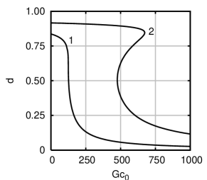
Figure 4: The width of the cloud $d$ versus ${\rm Gc}_{0}$ at ${\rm Gr}_{0}=150$ (line 1), ${\rm Gr}_{0}=500$ (line 2).

Let us discuss the dependence of the width of the particle cloud on the concentration parameter ${\rm Gc}_{0}$. At a relatively low ${\rm Gr}_{0}$ the width of the cloud $d$ monotonically decreases with the growth of ${\rm Gc}_{0}$ (see Fig. 4, line 1). This is related to the fact that the major part of the cloud is located in the ascending flow, hence, the larger ${\rm Gc}_{0}$, the higher effective density of the medium in this place. The higher density leads to a decrease of the buoyancy force and therefore to lowering of the flow velocity. The latter, in its turn, results in a decrease of the width of the dust cloud, in which the particles can remain in the suspended state.

At higher values of ${\rm Gr}_{0}$ the dependence of $d$ on ${\rm Gc}_{0}$ becomes more complex. Generally, in this case the growth of ${\rm Gc}$ also results in the decrease of the cloud width, but now in some range of ${\rm Gc}_{0}$ the dependence $d({\rm Gc}_{0})$ is no longer unique (see Fig. 4, line 2). At low ${\rm Gc}_{0}$ the growth of ${\rm Gc}_{0}$ only slightly influences the width of the cloud, but starting from some threshold value of ${\rm Gc}_{0}$, the drag force of the wide cloud becomes so strong that the flow is unable to keep it further. As a result, the width of a cloud decreases by a jump. If now, starting from a large value of ${\rm Gc}_{0}$, we decrease it, first, the cloud width varies insignificantly, but then at some critical value of concentration parameter the width of a cloud makes a jump to nearly the highest possible value for a given ${\rm Gr}_{0}$. Thus, the decrease of the cloud width with the change of particle concentration demonstrates a well pronounced hysteresis.

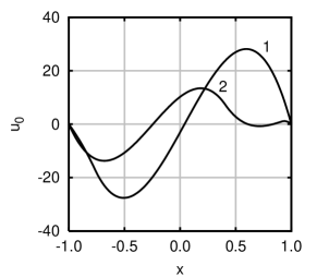
Figure 5: Velocity profiles for upper (line 1) and lower (line 2) branches of solutions at ${\rm Gr}_{0}=500$, ${\rm Gc}_{0}=600$.

In Fig. 5 the profiles of the fluid velocity at ${\rm Gr}_{0}=500$, ${\rm Gc}_{0}=600$ are plotted for upper (line 1) and lower (line 2) branches of possible steady states. It is seen, that for the upper branch the velocity profile only slightly differs from the usual cubic profile (21), but for the lower branch the flow in the domain occupied by the cloud is strongly suppressed, the total intensity of the flow is also low.

In Fig. 6 we plot a diagram defining a range of hysteresis existence on the plane ($\rm Gc_{0}$, $\rm Gr_{0}$). The solid lines divide the plane into two parts: larger and smaller ones. Any point of the larger part corresponds to only one solution (one root of a cloud width $d$ at fixed $\rm Gc_{0}$, $\rm Gr_{0}$), whereas in the smaller one, the hysteresis zone, there are three solutions (see Fig. 4). The solid lines, at which there exist two solutions, correspond to folds; the point where these lines intersect is a cusp with one solution. Inside the hysteresis zone, one of three solutions, namely, corresponding to the middle branch of a hysteresis curve $d({\rm Gc}_{0})$ in Fig. 4, is structurally unstable.

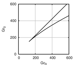
Figure 6: Hysteresis range on the parameter plane (${\rm Gc}_{0}$, ${\rm Gr}_{0}$).

IV.2 3.2. Linear stability analysis

IV.2.1 Formulation of stability problem

Let us investigate the stability of the basic steady state. We restrict our consideration to a fixed value of the Prandtl number ${\rm Pr}=1$, which corresponds to a typical case of particles, suspended in gaseous medium.

In order to formulate the stability problem, the governing equations (8)-(11) should be supplemented by necessary conditions at the rigid boundaries of the layer and continuity conditions at the borders of the dust cloud. At the rigid walls of the layer we impose the no slip condition for fluid velocity, and the condition of constant temperature:

$$x=\pm 1:\quad{\bf u}=0,\quad T=\pm 1.$$ (28)

The borders of the dust cloud, which are the surfaces of discontinuity for particle concentration, must satisfy the conditions of stress balance, the continuity of velocity, temperature, and energy flux. These conditions are the direct consequence of conservation laws for momentum, energy, and mass. Assuming that the borders of a dust cloud are deformable, the conditions at the interfaces are

$$x=x_{1,2}+\zeta_{1,2}: -[p]+\left[\varepsilon_{nn}\right]=0,\;[\varepsilon_{n\tau}]=0,$$ (29)

$$[{\bf u}]=0,\;[T]=0,\;\left[\frac{\partial T}{\partial n}\right]=0,$$

where $\zeta_{1}=\zeta_{1}(y,z,t)$, $\zeta_{2}=\zeta_{2}(y,z,t)$ are the deviations of concentration surfaces from the flat undisturbed shapes, and square brackets are used to denote the jump of a function $[f]=f_{2}-f_{1,3}$. Here the subscripts $1$, $2$, $3$ correspond to three zones of the flow: $1)$ $-1<x<x_{1}+\zeta_{1}$, $2)$ $x_{1}+\zeta_{1}<x<x_{2}+\zeta_{2}$, $3)$ $x_{2}+\zeta_{2}<x<1$. The unit normal $\bf n$ and tangential ${\bm{\tau}}_{1}$, ${\bm{\tau}}_{2}$ vectors to the surface are given by the relationships

$${\bf n}=\frac{{\bf e}_{x}-\nabla\zeta_{1,2}}{\sqrt{1+\left(\nabla\zeta_{1,2}\right)^{2}}},\;\;{\tau}_{1}=\frac{{\bf e}_{z}+{\bf e}_{x}\,{\bf e}_{z}\cdot\nabla\zeta_{1,2}}{\sqrt{1+\left({\bf e}_{z}\cdot\nabla\zeta_{1,2}\right)^{2}}},$$

$${\tau}_{2}={\bf n}\times{\tau}_{1}.$$

Here we introduce the orts ${\bf e}_{x}=(1,0,0)$, ${\bf e}_{y}=(0,1,0)$ of the axes $x$ and $y$, respectively. Both borders of the dust cloud are impervious to the particles, the velocity of any point of such border coincides with the Lagrangian velocity of a particle at this point. Hence, for surface deviations the following kinematic conditions are specified:

$$\frac{\partial\zeta_{1,2}}{\partial t}+{\bf u}_{p}\cdot\nabla\zeta_{1,2}={\bf u}_{p}\cdot{\bf e}_{x}.$$ (30)

Let the basic steady state be disturbed by introducing small perturbations of the velocity ${\bf v}$, pressure $q$, temperature $\vartheta$ and concentration $\phi$. Then we substitute the disturbed fields ${\bf u}_{0}+{\bf v}$, $p_{0}+q$, $T_{0}+\vartheta$, $\varphi_{0}+\phi$ into Eqs. (8)-(11). Neglecting squared and higher order terms with respect to perturbations, we obtain the equations for perturbations:

$$\frac{\partial{\bf v}}{\partial t}+{\bf u}_{0}\cdot\nabla{\bf v}+{\bf v}\cdot\nabla{\bf u}_{0} = -\nabla q+{\nabla}^{2}{\bf v}\mbox{}+{\rm Gr}\,\vartheta\,{\bf e}_{z}$$ (31)

$$\mbox{}-{\rm Gc}\,\phi\,{\bf e}_{z},$$

$$\frac{\partial\vartheta}{\partial t}+{\bf u}_{0}\cdot\nabla\vartheta+{\bf v}\cdot\nabla T_{0} = \frac{1}{\rm Pr}{\nabla}^{2}\vartheta,\quad{\rm div}\,{\bf v}=0,$$ (32)

$$\frac{\partial\phi}{\partial t}+\left({\bf u}_{0}-{\rm S}\,{\bf e}_{z}\right)\cdot\nabla\phi = 0,$$ (33)

where ${\bf u}_{0}=\left(0,0,u_{0}(x)\right)$.

The boundary conditions (28) take the form for perturbations:

$$x=\pm 1:\quad{\bf v}=0,\quad\vartheta=0.$$ (34)

Let us also assume the smallness of $\zeta_{1}$, $\zeta_{2}$. Then, the equations (31)-(33), boundary conditions (34) and conditions at deformable interfaces (29) reduced to those for undisturbed interfaces admit a transformation, which is analogous to the Squire transformation squire-33 and discussed below. Such a transformation allows us to reduce the full three-dimensional problem to a problem in two dimensions. We denote the $x$ and $z$ components of the velocity $\bf v$ by $u$ and $w$, respectively and analyze the stability of the basic steady state with respect to the two-dimensional perturbations in the form of transversal rolls. Thus, the solution can be written as normal modes

$$\left(\begin{array}[]{cccccc}u(x,z,t)\\ w(x,z,t)\\ q(x,z,t)\\ \vartheta(x,z,t)\\ \phi(x,z,t)\\ \zeta_{1,2}(z,t)\end{array}\right)=\left(\begin{array}[]{cccccc}\hat{u}(x)\\ \hat{w}(x)\\ \hat{q}(x)\\ \hat{\vartheta}(x)\\ \hat{\phi}(x)\\ \hat{\zeta}_{1,2}\end{array}\right)e^{\lambda t-ikz},$$ (35)

where $\lambda=\lambda_{r}+i\lambda_{i}$ is the complex growth rate, $k$ is the wave number, characterizing periodicity of perturbations along the $z$-axis.

Let us substitute the ansatz (35) into Eqs. (31)-(33). It follows from (33) that

$$\left\{\lambda-ik(u_{0}-{\rm S})\right\}\hat{\phi}=0,$$

which must be satisfied at every point of a layer occupied by particles. Since $u_{0}$ is a function of $x$ we assume that $\left\{\lambda-ik(u_{0}-{\rm S})\right\}\neq 0$, ${\hat{\phi}}=0$. As a result, in each of the three zones the problem is defined by the same set of amplitude equations:

$$\lambda\hat{u}-iku_{0}\hat{u} = -\hat{q}^{\prime}+\hat{u}^{\prime\prime}-k^{2}\hat{u},$$ (36)

$$\lambda\hat{w}-iku_{0}\hat{u}+u_{0}^{\prime}\hat{u} = ik\hat{q}+\hat{w}^{\prime\prime}-k^{2}\hat{w}+{\rm Gr}\hat{\vartheta},$$ (37)

$$\hat{u}^{\prime}-ik\hat{w} = 0,$$ (38)

$$\lambda\hat{\vartheta}-iku_{0}\hat{\vartheta}+\hat{u} = \frac{1}{\rm Pr}\left(\hat{\vartheta}^{\prime\prime}-k^{2}\hat{\vartheta}\right).$$ (39)

After linearization, the boundary conditions (34) and the conditions (29) at the pure liquid-suspension interface, i.e. at the borders of a dust cloud, written for the amplitudes of perturbations, take the form:

$$x=\pm 1: \hat{u}=0,\;\;\hat{w}=0,\;\;\hat{\vartheta}=0,$$ (40)

$$x=x_{1,2}: [\hat{q}]=0,\;\;[\hat{u}]=0,\;\;[\hat{w}]=0,$$ (41)

$$[\hat{w}^{\prime}]=-{\rm Gc}\,\hat{\zeta}_{1,2},\;\;[\hat{\vartheta}]=0,\;\;[\hat{\vartheta}^{\prime}]=0,$$

where $\hat{\zeta}_{1}$ and $\hat{\zeta}_{2}$ are obtained from Eqs. (30) together with (41) and are determined by the relations

$$x=x_{1}:\;\;\left\{\lambda-ik(u_{0}-{\rm S})\right\}\hat{\zeta}_{1}=\hat{u};\quad x=x_{2}:\;\;\lambda\hat{\zeta}_{2}=\hat{u}.$$ (42)

The conditions (40)-(42) are defined taking into account the following properties of the undisturbed velocity profile (IV.1): $[u_{0}]=0$, $[u_{0}^{\prime}]=0$, $[u_{0}^{\prime\prime}]={\rm Gc}$, and $u_{0}(x_{2})={\rm S}$.

The boundary value problem (36)-(42) is a spectral amplitude problem. The conditions of nontrivial solution define perturbation growth rate as a function of the parameters $\rm Gr$, $\rm Pr$, $\rm Gc$, $\rm S$ and $k$. The solution with $\lambda_{r}=0$ determines the neutral behavior and separates the regions of unstable modes with $\lambda_{r}>0$ from those of stable modes with $\lambda_{r}<0$.

In the particular case of ${\rm Gc}=0$, the particles have no influence on the fluid motion, and the boundary value problem (36)-(42) reduces to the stability analysis gershuni-zhuhovitsky-76 of a flow with the odd velocity profile (21). For ${\rm Pr}=1$, the instability appears above the critical value ${\rm Gr}_{min}=496.3$, which is reached at $k_{min}=1.404$, and corresponds to the monotonic (i.e. to the solution with zero imaginary part of the growth rate $\lambda_{i}=0$) “hydrodynamic” perturbations.

In the case of ${\rm Gc}\neq 0$, the problem admits analytical solution in the limit of short wavelength behavior for a small, but finite width of the dust cloud. In the general case, the boundary value problem (36)-(42) was treated numerically by the standard shooting and differential sweep methods, which gave very close agreement of the results.

IV.2.2 Thin dust cloud, short wavelength limit

In the case of a thin cloud, the parameter $d$ is small, and the problem can be simplified. The nonlinear algebraic equations (26), (27), defining the width of the cloud $d$ and the coordinate of its center $x_{c}$, can be solved explicitly with the accuracy $O\left(d^{2}\right)$:

$$x_{c}=\frac{1}{\sqrt{3}},\quad d=\frac{1}{3\sqrt{3}{\rm Gc}}\left({\rm Gr}-9\sqrt{3}{\rm S}\right).$$ (43)

In the limit of vanishing cloud width, when $d\to 0$, we obtain the lower threshold for the existence of a dust cloud ${\rm Gr}=9\sqrt{3}{\rm S}$, which is in agreement with the the value obtained above for an arbitrary value of $d$. It is clearly seen from (IV.1) that in this case the velocity profile coincides with (21). A thin cloud is located in the vicinity of the point at which the fluid velocity is maximal.

The short wavelength limit means that the wave number is large $k\to\infty$. Let us investigate the case of small, but finite values of $d$. Formally, this case corresponds to the limiting transition, when $d\to 0$, $k\to\infty$, but their product $kd$ is finite.

This particular case can be examined in the context of the auxiliary problem, in which the layers of pure fluid are semi-infinite and the dust cloud is in between these layers and has the finite width $2d$. It is convenient to treat the problem using the multi-scales technique.nayfeh-81 Let us introduce the “fast” coordinate $\xi=(x-x_{c})/\varepsilon$, where $\varepsilon=1/k$ is the small parameter. In terms of the fast coordinate the dust cloud occupies the finite region $-\Delta<\xi<\Delta$ with the center at the point $\xi=0$. Here $\Delta=kd$ is a semi-width of the cloud, measured in the units of the fast coordinate. The layers of pure fluid occupy the areas $-\infty<\xi<-\Delta$ and $\Delta<\xi<\infty$, respectively.

The boundary value problem (36)-(42) is rewritten in terms of the fast coordinate $\xi$. As a result we obtain the equations:

$$\varepsilon^{2}\lambda\hat{u}-i\varepsilon u_{0}\hat{u} = -\varepsilon\hat{q}^{\prime}+\hat{u}^{\prime\prime}-\hat{u},$$ (44)

$$\varepsilon^{2}\lambda\hat{w}-i\varepsilon u_{0}\hat{w}+\varepsilon^{2}u_{0}^{\prime}\hat{u} = i\varepsilon\hat{q}+\hat{w}^{\prime\prime}-\hat{w}$$ (45)

$$+\varepsilon^{2}{\rm Gr}\hat{\vartheta},$$

$$\hat{u}^{\prime}-i\hat{w} = 0,$$ (46)

$$\varepsilon^{2}\lambda\hat{\vartheta}-i\varepsilon u_{0}\hat{\vartheta}+\varepsilon^{2}\hat{u} = \frac{1}{{\rm Pr}}\left(\hat{\vartheta}^{\prime\prime}-\hat{\vartheta}\right),$$ (47)

which are the same for all three zones: 1) $-\infty<\xi<-\Delta$, 2) $-\Delta<\xi<\Delta$, 3) $\Delta<\xi<\infty$. We require that the functions $\hat{u}$, $\hat{w}$, $\hat{q}$, $\hat{\vartheta}$ must be bounded at $\xi=\pm\infty$. The conditions at the borders of the cloud are as follows:

$$\xi=\pm\Delta: [\hat{q}]=0,\;\;[\hat{u}]=0,\;\;[\hat{w}]=0,$$ (48)

$$[\hat{w}^{\prime}]=-\varepsilon{\rm Gc}\hat{\zeta}_{1,2},\;\;[\hat{\vartheta}]=0,\;\;[\hat{\vartheta}^{\prime}]=0,$$

$$\xi=-\Delta: \left\{\varepsilon\lambda-i(u_{0}-{\rm S})\right\}\hat{\zeta}_{1}=\varepsilon\hat{u},$$ (49)

$$\xi=\Delta: \lambda\hat{\zeta}_{2}=\hat{u},$$ (50)

where $\hat{\zeta}_{1}$ and $\hat{\zeta}_{2}$ refer to the points $\xi=-\Delta$ and $\xi=\Delta$, respectively.

For each zone the solution is sought as a power series in $\varepsilon$. Taking into account (43), we rewrite the velocity profile (IV.1) with the accuracy $O\left(\varepsilon^{3}\right)$:

$$u_{0}^{(1)} = {\rm S}-\varepsilon^{2}\left\{\frac{\rm Gr}{\sqrt{3}}\frac{(\xi+\Delta)^{2}}{2}+\Delta\left(\frac{\rm Gr}{\sqrt{3}}-{\rm Gc}\right)\left(\xi+\Delta\right)\right\},$$

$$u_{0}^{(2)} = {\rm S}-\varepsilon^{2}\left(\frac{\rm Gr}{\sqrt{3}}-{\rm Gc}\right)\left(\frac{\xi^{2}-\Delta^{2}}{2}\right),$$

$$u_{0}^{(3)} = {\rm S}-\varepsilon^{2}\left\{\frac{\rm Gr}{\sqrt{3}}\frac{(\xi-\Delta)^{2}}{2}-\Delta\left(\frac{\rm Gr}{\sqrt{3}}-{\rm Gc}\right)\left(\xi-\Delta\right)\right\}.$$

The boundary value problem (44)-(50) is the inner one with respect to the initial problem (36)-(42), which in its turn should be referred to as an outer one. Generally, the solutions of inner problem is matched to the outer one. However, this should not necessary be done in the present case since the solution of the inner problem (44)-(50) proves to be vanishing at $\xi=\pm\infty$.

The solution of the boundary value problem (44)-(50) is quite cumbersome and is not adduced here. Actually, the expressions for complex growth rates are of primary interest. In the zero order we obtain the trivial solution $\lambda^{(0)}=0$ and in higher orders we find the nonzero corrections to $\lambda^{(0)}$, corresponding (with accuracy up to the small terms of higher order) to two different types of deformation of the dust cloud borders $\hat{\zeta}_{1}=\pm\hat{\zeta}_{2}$:

$$\lambda^{(1)}=\pm ikd\,{\rm Gc}\,{\rm e}^{-2kd},\;\;\lambda_{r}^{(2)}=\mp kd\,{\rm Gc\,S}\left(1+2kd\right){\rm e}^{-2kd}.$$ (51)

One solution corresponds to deformation of the cloud borders in the “phase,” when $\hat{\zeta}_{1}=\hat{\zeta}_{2}$. This solution is stable since the real part of the growth rate is negative. In the other solution, allowing for deformation of the cloud borders in the “anti-phase,” when $\hat{\zeta}_{1}=-\hat{\zeta}_{2}$, the real part of the growth rate is positive, and hence this solution is unstable. In both solutions the imaginary part of the growth rate is nonzero suggesting that the behavior of the system is oscillatory.

Note, that the obtained result is true for any nontrivial values the parameters $\rm Gc$ and $\rm S$. Thus, we conclude that the dust cloud of a small, but finite width is unstable with respect to short wavelength perturbations.

IV.2.3 Dust cloud of an arbitrary width

Let us proceed to the discussion of general numerical results, obtained for a cloud of arbitrary width $d$, and consider the case ${\rm S}=1$.

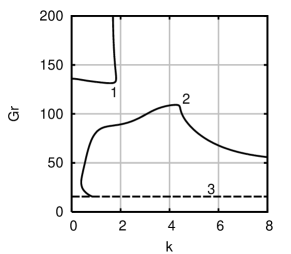
Figure 7: Neutral curves (line 1 and 2), plotted for ${\rm Gc}=100$, ${\rm S}=1$. Regions of unstable behavior are above the line 1 and under the line 2. Line ${\rm Gr}=9\sqrt{3}{\rm S}$ (line 3) corresponds to a cloud of the vanishing width.

The neutral curves for a fixed value of the concentration parameter ${\rm Gc}=100$ are presented in Fig. 7. The instability regions are above the curve $1$ (between the curve $1$ and the line $k=0$) and under the curve $2$ (between the curves $2$ and $3$). Curve $3$ is a straight line at which ${\rm Gr}=9\sqrt{3}{\rm S}$. This line defines the area of existence of a dust cloud and corresponds to a dust cloud of zero width. The cloud exists in the domain that is above this line. As can be seen, there is a narrow range of values of $\rm Gr$, where the system is stable. The results (51), valid for a thin cloud in the short wavelength limit, are in agreement with those obtained from numerical solution to the general boundary value problem (36)-(42). However, it is obvious from Fig. 7, that the short wavelength instability is not “the most dangerous”: although in some range of governing parameters the flow is stable with respect to short waves, but yet for all possible values of the cloud width $d$ there exist unstable two-dimensional perturbations in the form of transversal rolls with finite values of $k$. It is interesting to note, that the steady state in the case of a thin cloud is unstable with respect to perturbations with any wave number $k$ larger than some critical value.

The global minimum of the curve $1$ and the global maximum of the curve $2$ over $k\geq 0$ in Fig. 7 are characterized by the critical values of the Grashof number: ${\rm Gr}_{min}$, ${\rm Gr}_{max}$, which are reached at the values of the wave number $k_{min}$, $k_{max}$ respectively. Let us discuss the dependence of these critical parameters on the concentration parameter $\rm Gc$. Figure 8 gives the stability diagram on the plane ($\rm Gc$, $\rm Gr$). The stability region is under the line $1$ and above the line $2$. Note, that the curves $1$ and $2$ refer to the upper and the lower branches of the dependence $d\left({\rm Gc}\right)$, respectively (see Fig. 4). This becomes important for distinguishing between stability regions for the upper and lower branches in the hysteresis zone (Fig. 6), bounded by lines 4 and 5: the stability region of the upper branch is defined by the curve 1, for the lower branch it is defined by the curve 2. As before, the line $3$ is a line determining the region of a cloud of vanishing width, at which ${\rm Gr}=9\sqrt{3}{\rm S}$.

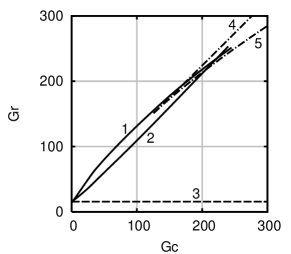
Figure 8: Stability curves for the upper (line 1) and the lower (line 2) branches of the dependence $d\left({\rm Gc}\right)$ on a plane ($\rm Gc$, $\rm Gr$) at ${\rm S}=1$. The stability regions are under the line 1 and above the line 2. Line 3 is the line ${\rm Gr}=9\sqrt{3}{\rm S}$; lines 4 and 5 represent bounds of the hysteresis zone (see Fig. 6).

It should be noticed that the section of the straight line ${\rm Gc}=0$, at $9\sqrt{3}<{\rm Gr}<496.3$ also refers to a stability region. A piece of this line, corresponding to the values $0\leq{\rm Gr}<9\sqrt{3}$ is stable as well, however, the basic steady state in this case is completely free of particles, i.e. a dust cloud is absent.

The variation of $k_{min}$, $k_{max}$ with the concentration parameter $\rm Gc$ is shown in Fig. 9. The imaginary parts of growth rates corresponding to these solutions are nonzero, which means that this “concentration” mode is oscillatory. The hydrodynamic perturbations are not the most dangerous for our particular value of sedimentation parameter $\rm S$, their stability bound lies much higher than the lines $1$ and $2$. Of special note is the dependence $k_{min}({\rm Gc})$ at relatively small values of the concentration parameter $\rm Gc$. It is seen, that for not very large values of $\rm Gc$ the wave number $k_{min}$ is rather small, i.e. the system demonstrates a nearly long wavelength behavior.

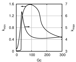
Figure 9: Critical wave numbers $k_{min}$, $k_{max}$ as functions of ${\rm Gc}$ at ${\rm S}=1$.

With the increase of the sedimentation parameter $\rm S$ the region of hysteresis wedge shifts to the region of larger values of $\rm Gr$ and $\rm Gc$. Fig. 10 presents the stability diagram for the case ${\rm S}=5$. The stability curves $1$ and $2$ do not undergo any qualitative changes. However, in contrast to the case ${\rm S}=1$, the concentration mode is in competition with the hydrodynamic mode: there appears the range of values of $\rm Gc$, at which the hydrodynamic perturbations (line 6) become the most dangerous for the upper branch of the dependence $d({\rm Gc})$. With increase of $\rm S$ this range grows, reducing the total stability region. In the hysteresis zone line 6 sticks to the line 5: the upper branch becomes unstable here. In comparison with the case ${\rm Gc}=0$, the hydrodynamic mode is no longer monotonic. Indeed, the monotonic character of hydrodynamic perturbations is specified gershuni-zhuhovitsky-76 by the symmetry of the velocity profile $u_{0}$. In our case, as it follows from (IV.1), the symmetry of $u_{0}$ is broken at any value ${\rm Gc}\neq 0$.

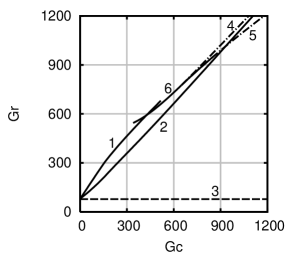
Figure 10: Stability curves for the upper (lines 1 and 6) and the lower (line 2) branches of $d\left({\rm Gc}\right)$ on a plane ($\rm Gc$, $\rm Gr$). The stability regions are under the line 1 and 6 and above the line 2. Line 3 is the line ${\rm Gr}=9\sqrt{3}{\rm S}$; lines 4 and 5 represent bounds of the hysteresis zone.

IV.2.4 Arbitrary three-dimensional perturbations

It was mentioned before, that after linearization Eqs. (31)-(33), boundary conditions (34) and the conditions at the borders of the dust cloud (29) admit a transformation, which is analogous to the Squire transformation.squire-33 Under such a transformation the Prandtl number $\rm Pr$ does not change, whereas the parameters $\rm Gr$, $\rm Gc$, and $\rm S$ transform according to the following rule:

$${\rm Gr}=\frac{k_{z}}{k}{\rm Gr^{\prime}},\quad{\rm Gc}=\frac{k_{z}}{k}{\rm Gc^{\prime}},\quad{\rm S}=\frac{k_{z}}{k}{\rm S^{\prime}},$$ (52)

where $\rm Gr$, $\rm Gc$, $\rm S$ are the parameters of the two-dimensional problem and $\rm Gr^{\prime}$, $\rm Gc^{\prime}$, $\rm S^{\prime}$ are the corresponding parameters of the full three-dimensional problem; $k_{y}$ and $k_{z}$ are the wave numbers along the axes $y$ and $z$, respectively; $k^{2}=k_{y}^{2}+k_{z}^{2}$. Note, that at any given value $k_{z}/k$ the parameters of the two-dimensional problem $\rm Gr$, $\rm Gc$, $\rm S$ are always less than those of the three-dimensional problem. However, this fact does not imply that two-dimensional perturbations are the most dangerous.

Let us introduce the parameter, describing deviation of arbitrary three-dimensional perturbations from the two-dimensional perturbations in the form of transverse rolls (35), namely the angle between the wave vector ${\bf k}=(0,k_{y},k_{z})$, which generally lies in the plane $y$-$z$, and the $z$-axis. If we denote the cosine of this angle by $\alpha$, then it follows from (52)

$${\rm Gr}^{\prime}=\frac{\rm Gr}{\alpha},\quad{\rm Gc}^{\prime}=\frac{\rm Gc}{\alpha},\quad{\rm S}^{\prime}=\frac{\rm S}{\alpha}.$$

The greatest distinction of arbitrary three-dimensional perturbations from transversal rolls (35) corresponds to the limiting case of longitudinal rolls, when $\alpha=0$ $(k_{z}=0$, $k\neq 0)$. The perturbations of this kind are often called the “helical” perturbations, since the trajectory of a fluid element in such a flow looks like a helix. The motion of a fluid particle can be considered as a sum of two different forms of motion: first, the particle moves circle-wise inside the longitudinal roll, second, it is carried along the roll with the velocity $u_{0}+u$.

Thus, at given $\alpha$ the diagram of stability with respect to arbitrary three-dimensional perturbations can be obtained from that of two-dimensional perturbations (35) by rescaling $\rm Gr$ and $\rm Gc$ by a factor of $1/\alpha$. It is important to note, that the parameter $\rm S$ is also transformed.

The linear stability analysis, performed with respect to two-dimensional perturbations (35) for $\rm S$ from $1$ up to $5$, allows us to investigate the influence of three-dimensional perturbations with $\alpha$ in the range from $0.2$ up to $1$ for ${\rm S}=5$. It turns out, that in this range the most dangerous are the perturbations in the form of transversal rolls.

Further, it can be explicitly shown, that the limiting case of the longitudinal rolls (helical perturbations), when $\alpha=0$ $(k_{z}=0$, $k\neq 0)$, does not cause instability. Indeed, as it follows from Eqs. (31)-(34) and linearized form of conditions (29), (30), this particular case is described by the following boundary value problem (the equations are the same for each of three zones):

$$\lambda\hat{u} = -\hat{q}^{\prime}+\hat{u}^{\prime\prime}-k_{y}^{2}\hat{u},$$ (53)

$$\lambda\hat{v} = ik_{y}\hat{q}+\hat{v}^{\prime\prime}-k_{y}^{2}\hat{v},$$ (54)

$$\hat{u}^{\prime}-ik_{y}\hat{v} = 0,$$ (55)

$$\lambda\hat{w}+u_{0}^{\prime}\hat{u} = \hat{w}^{\prime\prime}-k_{y}^{2}\hat{w}+{\rm Gr}\hat{\vartheta},$$ (56)

$$\lambda\hat{\vartheta}+\hat{u} = \frac{1}{\rm Pr}\left(\hat{\vartheta}^{\prime\prime}-k_{y}^{2}\hat{\vartheta}\right),$$ (57)

$$x=\pm 1: \hat{u}=0,\;\;\hat{v}=0,\;\;\hat{w}=0,\;\;\hat{\vartheta}=0,$$ (58)

$$x=x_{1,2}: [\hat{q}]=0,\;\;[\hat{u}]=0,\;\;[\hat{v}]=0,\;\;[\hat{\vartheta}]=0,$$ (59)

$$[\hat{\vartheta}^{\prime}]=0,\;\;[\hat{w}]=0,\;\;[\hat{w}^{\prime}]=-{\rm Gc}\,\hat{\zeta}_{1,2},$$

$$\lambda\hat{\zeta}_{1,2}=\hat{u}.$$

The problem for the fields $\hat{u}$ and $\hat{v}$ splits off and can be treated independently. Excluding the pressure $\hat{q}$ from Eqs. (53)-(55) and taking into account the continuity of $\hat{u}$ and $\hat{v}$ at the points $x_{1}$ and $x_{2}$, we obtain the following boundary value problem:

$$\lambda(\hat{v}^{\prime\prime}-k_{y}^{2}\hat{v}) = \hat{v}^{IV}-2k_{y}^{2}\hat{v}^{\prime\prime}+k_{y}^{4}\hat{v},$$ (60)

$$x=\pm 1:\;\;\hat{v} = 0,\;\;\hat{v}^{\prime}=0.$$ (61)

Let us multiply Eq. (60) by the complex conjugate $\hat{v}^{*}$ and integrate by parts across the layer. Taking into account (61), after elementary calculations we obtain

$$\lambda=-\frac{\left<\left|\hat{v}^{\prime\prime}\right|^{2}+2k_{y}^{2}\left|\hat{v}^{\prime}\right|^{2}+k_{y}^{4}\left|\hat{v}\right|^{2}\right>}{\left<\left|\hat{v}^{\prime}\right|^{2}+k_{y}^{2}\left|\hat{v}\right|^{2}\right>}<0,$$

where $\left<\ldots\right>=\int_{-1}^{1}\ldots\,dx$. Since the problem (60)-(61) describes perturbations in a quiescent viscous uniform fluid, it cannot give birth to instability: the growth rate is proved to be real and negatively defined; the perturbations monotonically decrease with time, and, therefore, one should look for a mode with $\hat{v}=0$. Hence, with account of incompressibility relation (55), the boundary conditions (58) for $\hat{u}$ and continuity of this field at the points $x_{1}$ and $x_{2}$ we obtain $\hat{u}=0$.

Since $\hat{u}=0$, equation (57) corresponds to diffusion of $\hat{\vartheta}$ in motionless fluid, and therefore, from analogous consideration we conclude that perturbations decrease. Hence, the mode with $\hat{\vartheta}=0$ is to be found. As it follows from the condition (59) for $\hat{\zeta_{1}}$ and $\hat{\zeta_{2}}$, the solution with $\lambda\neq 0$ is possible only if $\hat{\zeta_{1}}=0$ and $\hat{\zeta_{2}}=0$. Consequently, $\hat{w}$ and its derivative are continuous at the points $x_{1}$, $x_{2}$, and the problem for $\hat{w}$ coincides with the problem for $\hat{\vartheta}$ with the rescaled time $t\,{\rm Pr}^{-1}$. Thus, for any values of governing parameters the basic state is proved to be stable with respect to perturbations in the form of longitudinal rolls.

V Conclusions

The interaction of the vortex buoyancy convective flow laden with particles of dust has been investigated in the case when the volume concentration of the solid phase is small. Under these conditions the particles are partially carried away by the flow, but due to sedimentation their velocity differs from the velocity of a fluid. At sufficiently intensive thermal convection some portion of the particles can be captured by the flow, which eventually results in formation of a cloud of dust.

If mass concentration of the particles is rather small, the particles do not influence the flow and the study of the formation of a dust cloud is reduced to a kinematic problem. The size of the dust cloud captured by the convective vortex monotonically increases with the growth of the thermal Grashof number from some threshold value ${\rm Gr_{*}}$. At the values ${{\rm Gr}<{\rm Gr}_{*}}$, the formation of a steady cloud is impossible: sooner or later all the particles settle on the bottom of a cavity. This critical value of the Grashof number is determined by the cavity shape and thermal boundary conditions and is also proportional to the sedimentation parameter ${\rm S}$. The calculations for the case of an infinite vertical layer heated from the sidewalls give ${\rm Gr}_{*}=9\sqrt{3}{\rm S}$.

With the increase of mass concentration of the particles their influence on the flow becomes significant. This happens when relative variations of mass concentration are comparable with the Boussinesq nonisothermality parameter $\beta\theta$. Generally, the growth of mass concentration results in the decrease of flow intensity. Energy of the flow is partly consumed on the particle motion against the gravity and on the motion of particles together with the descending flow. This energy is not returned to the flow completely because of the dissipative loss. The calculations show that the interaction of the particles with the convective flow can lead to the hysteresis phenomena. Different flow patterns can arise at the same values of the governing parameters: the modes, in which a comparatively small dust cloud strongly suppresses the ascending flow and the modes developing at comparatively large cloud when the density inhomogeneities are low and the suppression effect is insignificant.

The linear stability of the basic steady state in the form of a dust cloud in an infinite layer, heated from sidewalls, has been investigated. It is shown, that in a relatively narrow range of the values of governing parameters this state is stable. Based on the results of the stability analysis, we can infer that in the typical case of a closed cavity the steady state with a relatively large dust cloud is most likely to have a larger range of stability. In the case of an infinite layer such a steady state is broken by long wavelength perturbations. Obviously, such perturbations cannot arise in a closed container of a finite size.

The performed investigation demonstrates that the described effects of two-way interaction of fluid and particles can exist in natural environment or be realized experimentally. The values of the sedimentation parameter ${\rm S}$ of order $1$, used in the linear stability analysis, correspond, for example, to the case of rather fine particles of dust with $r_{p}\sim 10^{-4}~{}{\rm cm}$, suspended under gravity in a gaseous medium filling a laboratory-scale container $L\sim 1~{}{\rm cm}$ ($r_{p}/L\sim 10^{-4}$, $\delta\sim 10^{3}$, ${\rm Ga}\sim 10^{5}$). The developed theory is quite general and can be applied to describe similar effects not only in dusty media, but also in aerosols, liquids laden with small solid particles, and biological species in aqueous media.

VI Acknowledgments

The research was partially supported by INTAS (Grant No. 2000-0617) and CRDF (Grant No. PE-009-0), which are gratefully acknowledged.

References

- (1) F. A. Williams, Combustion Theory (Benjamin-Cummings, Menlo Park, 1985).
- (2) S. Peters, Turbulent Combustion (University Press, Cambridge, 2000).
- (3) A. J. Koch and H. Meinhardt, “Biological pattern formation: from basic mechanisms to complex structures,” Rev. Mod. Phys. 66, 1481 (1984).
- (4) E. R. Abraham, “The generation of plankton patchiness by turbulent stirring,” Nature 391, 577 (1998).
- (5) P. A. del Giorgio and C. M. Duarte, “Respiration in the open ocean,” Nature 420, 379 (2002).
- (6) J. M. Ottino, The Kinematics of Mixing: Stretching, Chaos, and Transport (University Press, Cambridge, 1989).
- (7) S. L. Soo, Fluid Dynamics of Multiphase Systems (Blaisdell, Waltham, MA, 1967).
- (8) F. E. Marble, “Dynamics of dusty gases,” Annu. Rev. Fluid Mech. 2, 397, (1970).
- (9) M. R. Maxey, “On the advection of spherical and non-spherical particles in a non-uniform flow,” Philos. Trans. R. Soc. London, Ser. A 333, 289 (1990).
- (10) M. R. Maxey and J. J. Riley, “Equation of motion for small rigid sphere in a non-uniform flow,” Phys. Fluids 26, 883 (1983).
- (11) H. Stommel, “Trajectories of small bodies sinking slowly through convective cells,” J. Mar. Res. 8, 24 (1949).
- (12) B. Simon and Y. Pomeau, “Free and guided convection in evaporating layers of aqueous solutions of sucrose. Transport and sedimentation of solid particles,” Phys. Fluids A 3, 380 (1991).
- (13) K. Anderson, S. Sundaresan, and R. Jackson, “Instabilities and the formation of bubbles in fluidized beds,” J. Fluid Mech. 303, 327 (1995).
- (14) C. Pasquero, A. Provenzale, and E.A. Spiegel, “Suspension and fall of heavy particles in random two-dimensional field,” Phys. Rev. Lett. 91, 054502 (2003).
- (15) K.-K. Tio, A. Liñán, J. C. Lasheras, and A. M. Gañán-Calvo, “On the dynamics of buoyant and heavy particles in a periodic Stuart vortex flow,” J. Fluid Mech. 254, 671 (1993).
- (16) O. A. Druzhinin, “Dynamics of concentration and vorticity modification in a cellular flow laden with solid heavy particles,” Phys. Fluids 7, 2132 (1995).
- (17) O. A. Druzhinin, “On the two-way interaction in two-dimensional particle-laden flows: the accumulation of particles and flow modification,” J. Fluid Mech. 297, 49 (1995).
- (18) D. Schwabe and S. Frank, “Particle accumulation structures (PAS) in the toroidal thermocapillary vortex of a floating zone – model for a step in planet formation?” Adv. Space Res. 23, 1191 (1999).
- (19) M. R. Maxey and S. Corrsin, “Gravitational settling of aerosol particles in randomly oriented cellular flow fields,” J. Atmos. Sci. 43, 1112 (1986).
- (20) M. R. Maxey, “The motion of small spherical particles in a cellular flow field,” Phys. Fluids 30, 1915 (1987).
- (21) J. Dávila and J. C. R. Hunt, “Settling of small particles near vortices and in turbulence,” J. Fluid Mech. 440, 117 (2001).
- (22) P. J. Thomas, “On the influence of the Basset history force on the motion of a particle through a fluid,” Phys. Fluids A 4, 2090 (1992).
- (23) O. A. Druzhinin and L. A. Ostrovsky, “The influence of Basset force on particle dynamics in two-dimensional flows,” Physica D 76, 34 (1994).
- (24) A. N. Yannacopoulos, G. Rowlands, and G. P. King, “Influence of particle inertia and Basset force on tracer dynamics: analytic results in the small inertia limit,” Phys. Rev. E 55, 4148 (1997).
- (25) N. Mordant and J.-F. Pinton, “Velocity measurement of a settling sphere,” Eur. Phys. J. B 18, 343 (2000).
- (26) V. Armenio and V. Fiorotto, “The importance of the forces acting on particles in turbulent flows,” Phys. Fluids 11, 2437 (2001).
- (27) F. Candelier, J. R. Angilella, and M. Souhar, “On the effect of the Boussinesq-Basset force on the radial migration of a Stokes particle in a vortex,” Phys. Fluids 16, 1765 (2004).
- (28) P. G. Saffman, “On the stability of laminar flow of a dusty gas,” J. Fluid Mech. 13, 120 (1962).
- (29) D. H. Michael, “The stability of plane Poiseuille flow of a dusty gas,” J. Fluid Mech. 18, 19 (1964).
- (30) J. T. C. Liu, “On the hydrodynamic stability of parallel dusty gas flows,” Phys. Fluids 8,1939 (1965).
- (31) E. B. Isakov and V. Ya. Rudyak, “Stability of rarefied dusty gas and suspension flows in a plane channel,” Fluid Dynamics 30, 708 (1995).
- (32) V. Ya. Rudyak, E. B. Isakov, and E. C. Bord, “Hydrodynamic stability of the Poiseuille flow of dispersed fluid,” J. Aerosol Sci. 28, 53 (1996).
- (33) D. A. Drew, “Lift-generated instability of the plane Couette flow of a particle-fluid mixture,” Phys. Fluids 18, 935 (1975).
- (34) O. Dementiev, “Stability of steady-state flow of a liquid with a heavy impurity,” Zeitschrift für angewandte Mathematik und Mechanik 76, 113 (1996).
- (35) O. N. Dement’ev, “Effect of convection on the stability of a liquid with a nonuniformly distributed heavy admixture,” J. Appl. Mech. Techn. Phys. 41, 923 (2000).
- (36) D. V. Lyubimov, D. A. Bratsun, T. P. Lyubimova, and B. Roux, “Influence of gravitational precipitation of solid particles on the thermal buoyancy convection,” Adv. Space Res. 22, 1267 (1998).
- (37) R. I. Nigmatulin, Dynamics of Multiphase Media (Hemisphere, New York, 1991).
- (38) G. Z. Gershuni and E. M. Zhukhovitsky, Convective Stability of Incompressible Fluid (Keter Press, Jerusalem, 1976).
- (39) H. B. Squire, “On the stability of three-dimensional disturbances of viscous fluid flow between parallel walls,” Proc. R. Soc. London, Ser. A 142, 621 (1933).
- (40) A. H. Nayfeh, Introduction to Perturbation Techniques (Wiley & Sons, New York, 1981).