Simplified Variational Principles for Barotropic Magnetohydrodynamics

Abstract

Variational principles for magnetohydrodynamics were introduced by previous authors both in Lagrangian and Eulerian form. In this paper we introduce simpler Eulerian variational principles from which all the relevant equations of barotropic magnetohydrodynamics can be derived. The variational principle is given in terms of six independent functions for non-stationary barotropic flows and three independent functions for stationary barotropic flows. This is less then the seven variables which appear in the standard equations of barotropic magnetohydrodynamics which are the magnetic field $\vec{B}$ the velocity field $\vec{v}$ and the density $\rho$.

The equations obtained for non-stationary barotropic magnetohydrodynamics resemble the equations of Frenkel, Levich & Stilman [2]. The connection between the Hamiltonian formalism introduced in [2] and the present Lagrangian formalism (with Eulerian variables) will be discussed.

Finally the relations between barotropic magnetohydrodynamics topological constants and the functions of the present formalism will be elucidated.

Keywords: Magnetohydrodynamics, Variational principles

PACS number(s): 47.65.+a

1 Introduction

Variational principles for magnetohydrodynamics were introduced by previous authors both in Lagrangian and Eulerian form. Sturrock [3] has discussed in his book a Lagrangian variational formalism for magnetohydrodynamics. Vladimirov and Moffatt [4] in a series of papers have discussed an Eulerian variational principle for incompressible magnetohydrodynamics. However, their variational principle contained three more functions in addition to the seven variables which appear in the standard equations of magnetohydrodynamics which are the magnetic field $\vec{B}$ the velocity field $\vec{v}$ and the density $\rho$. Kats [5] has generalized Moffatt’s work for compressible non barotropic flows but without reducing the number of functions and the computational load. Moreover, Kats has shown that the variables he suggested can be utilized to describe the motion of arbitrary discontinuity surfaces [6, 7]. Sakurai [8] has introduced a two function Eulerian variational principle for force-free magnetohydrodynamics and used it as a basis of a numerical scheme, his method is discussed in a book by Sturrock [3]. A method of solving the equations for those two variables was introduced by Yang, Sturrock & Antiochos [9]. In this work we will combine the Lagrangian of Sturrock [3] with the Lagrangian of Sakurai [8] to obtain an Eulerian Lagrangian principle which will depend on only six functions. The variational derivative of this Lagrangian will give us all the equations needed to describe barotropic magnetohydrodynamics without any additional constraints. The equations obtained resemble the equations of Frenkel, Levich & Stilman [2] (see also [10]). The connection between the Hamiltonian formalism introduced in [2] and the present Lagrangian formalism (with Eulerian variables) will be discussed. Furthermore, we will show that for stationary flows three functions will suffice in order to describe a Lagrangian principle for barotropic magnetohydrodynamics. The non-singlevaluedness of the functions appearing in the reduced representation of barotropic magnetohydrodynamics will be discussed in particular with connection to the topological invariants of magnetic and cross helicities. It will be shown how the conservation of cross helicity can be easily generated using the Noether theorem and the variables introduced in this paper.

Due to space limitations this paper is concerned only with barotropic magnetohydrodynamics. Variational principles of non barotropic magnetohydrodynamics can be found in the work of Bekenstein & Oron [11] in terms of 15 functions and V.A. Kats [5] in terms of 20 functions. The authors of this paper suspect that this number can be somewhat reduced. Moreover, A. V. Kats in a remarkable paper [18] (section IV,E) has shown that there is a large symmetry group (gauge freedom) associated with the choice of those functions, this implies that the number of degrees of freedom can be reduced.

We anticipate applications of this study both to linear and non-linear stability analysis of known barotropic magnetohydrodynamic configurations [12, 13] and for designing efficient numerical schemes for integrating the equations of fluid dynamics and magnetohydrodynamics [14, 15, 16, 17].

The plan of this paper is as follows: first we introduce the standard notations and equations of barotropic magnetohydrodynamics. Next we review the Lagrangian variational principle of barotropic magnetohydrodynamics. This is followed by a review of the Eulerian variational principles of force-free magnetohydrodynamics. After those introductory sections we will present the six function Eulerian variational principles for non-stationary magnetohydrodynamics. A derivation of the canonical momenta of the generalized coordinates appearing in the Lagrangian allows us to derive the system’s Hamiltonian which resembles the Hamiltonian introduced by Frenkel, Levich & Stilman [2]. This is followed by the derivation of a variational principle for stationary magnetohydrodynamics. The discussion related to the magnetohydrodynamic topological constants concludes our paper.

2 The standard formulation of barotropic magnetohydrodynamics

2.1 Basic equations

The standard set of equations solved for barotropic magnetohydrodynamics are given below:

$$\frac{\partial{\vec{B}}}{\partial t}=\vec{\nabla}\times(\vec{v}\times\vec{B}),$$ (1)

$$\vec{\nabla}\cdot\vec{B}=0,$$ (2)

$$\frac{\partial{\rho}}{\partial t}+\vec{\nabla}\cdot(\rho\vec{v})=0,$$ (3)

$$\rho\frac{d\vec{v}}{dt}=\rho(\frac{\partial\vec{v}}{\partial t}+(\vec{v}\cdot\vec{\nabla})\vec{v})=-\vec{\nabla}p(\rho)+\frac{(\vec{\nabla}\times\vec{B})\times\vec{B}}{4\pi}.$$ (4)

The following notations are utilized: $\frac{\partial}{\partial t}$ is the temporal derivative, $\frac{d}{dt}$ is the temporal material derivative and $\vec{\nabla}$ has its standard meaning in vector calculus. $\vec{B}$ is the magnetic field vector, $\vec{v}$ is the velocity field vector and $\rho$ is the fluid density. Finally $p(\rho)$ is the pressure which we assume depends on the density alone (barotropic case). The justification for those equations and the conditions under which they apply can be found in standard books on magnetohydrodynamics (see for example [3]). Equation (1) describes the fact that the magnetic field lines are moving with the fluid elements (”frozen” magnetic field lines), equation (2) describes the fact that the magnetic field is solenoidal, equation (3) describes the conservation of mass and equation (4) is the Euler equation for a fluid in which both pressure and Lorentz magnetic forces apply. The term:

$$\vec{J}=\frac{\vec{\nabla}\times\vec{B}}{4\pi},$$ (5)

is the electric current density which is not connected to any mass flow. The number of independent variables for which one needs to solve is seven ($\vec{v},\vec{B},\rho$) and the number of equations (1,3,4) is also seven. Notice that equation (2) is a condition on the initial $\vec{B}$ field and is satisfied automatically for any other time due to equation (1). Also notice that $p(\rho)$ is not a variable rather it is a given function of $\rho$.

2.2 Lagrangian variational principle of magnetohydrodynamics

A Lagrangian variational principle for barotropic magnetohydrodynamics has been discussed by a number of authors (see for example [3]) and an outline of this approach is given below. Consider the action:

$$A \equiv \int{\cal L}d^{3}xdt,$$

$${\cal L} \equiv \rho(\frac{1}{2}\vec{v}^{2}-\varepsilon(\rho))-\frac{\vec{B}^{2}}{8\pi},$$ (6)

in which $\varepsilon(\rho)$ is the specific internal energy. A variation in any quantity $F$ for a fixed position $\vec{r}$ is denoted as $\delta F$ hence:

$$\delta A = \int\delta{\cal L}d^{3}xdt,$$

$$\delta{\cal L} = \delta\rho(\frac{1}{2}\vec{v}^{2}-w(\rho))+\rho\vec{v}\cdot\delta\vec{v}-\frac{\vec{B}\cdot\delta\vec{B}}{4\pi},$$ (7)

in which $w=\frac{\partial(\varepsilon\rho)}{\partial\rho}$ is the specific enthalpy.

A change in a position of a fluid element located at a position $\vec{r}$ at time $t$ is given by $\vec{\xi}(\vec{r},t)$. A mass conserving variation of $\rho$ takes the form:

$$\delta\rho=-\vec{\nabla}\cdot(\rho\vec{\xi})$$ (8)

and a magnetic flux conserving variation takes the form:

$$\delta\vec{B}=\vec{\nabla}\times(\vec{\xi}\times\vec{B}).$$ (9)

A change involving both a local variation coupled with a change of element position of the quantity $F$ is given by:

$$\Delta F=\delta F+(\vec{\xi}\cdot\vec{\nabla})F,$$ (10)

hence

$$\Delta\vec{v}=\delta\vec{v}+(\vec{\xi}\cdot\vec{\nabla})\vec{v}.$$ (11)

However, since:

$$\Delta\vec{v}=\Delta\frac{d\vec{r}}{dt}=\frac{d\Delta\vec{r}}{dt}=\frac{d\vec{\xi}}{dt}.$$ (12)

We obtain:

$$\delta\vec{v}=\frac{d\vec{\xi}}{dt}-(\vec{\xi}\cdot\vec{\nabla})\vec{v}=\frac{\partial\vec{\xi}}{\partial t}+(\vec{v}\cdot\vec{\nabla})\vec{\xi}-(\vec{\xi}\cdot\vec{\nabla})\vec{v}.$$ (13)

Introducing the result of equations (8,9,13) into equation (7) and integrating by parts we arrive at the result:

$$\delta A = \int d^{3}x\rho\vec{v}\cdot\vec{\xi}|^{t_{1}}_{t_{0}}$$ (14)

$$+ \int dt\{\oint d\vec{S}\cdot[-\rho\vec{\xi}(\frac{1}{2}\vec{v}^{2}-w(\rho))+\rho\vec{v}(\vec{v}\cdot\vec{\xi})+\frac{1}{4\pi}\vec{B}\times(\vec{\xi}\times\vec{B})]$$

$$+ \int d^{3}x\vec{\xi}\cdot[-\rho\vec{\nabla}w-\frac{\partial(\rho\vec{v})}{\partial t}-\frac{\partial(\rho\vec{v}v_{k})}{\partial x_{k}}-\frac{1}{4\pi}\vec{B}\times(\vec{\nabla}\times\vec{B})]\},$$

in which a summation convention is assumed. Taking into account the continuity equation (3) we obtain:

$$\delta A = \int d^{3}x\rho\vec{v}\cdot\vec{\xi}|^{t_{1}}_{t_{0}}$$ (15)

$$+ \int dt\{\oint d\vec{S}\cdot[-\rho\vec{\xi}(\frac{1}{2}\vec{v}^{2}-w(\rho))+\rho\vec{v}(\vec{v}\cdot\vec{\xi})+\frac{1}{4\pi}\vec{B}\times(\vec{\xi}\times\vec{B})]$$

$$+ \int d^{3}x\vec{\xi}\cdot[-\rho\vec{\nabla}w-\rho\frac{\partial\vec{v}}{\partial t}-\rho(\vec{v}\cdot\vec{\nabla})\vec{v}-\frac{1}{4\pi}\vec{B}\times(\vec{\nabla}\times\vec{B})]\},$$

hence we see that if $\delta A=0$ for a $\vec{\xi}$ vanishing at the initial and final times and on the surface of the domain but otherwise arbitrary then Euler’s equation (4) is satisfied (taking into account that in the barotropic case $\vec{\nabla}w=\frac{\vec{\nabla}p}{\rho}$).

Although the variational principle does give us the correct dynamical equation for an arbitrary $\vec{\xi}$, it has the following deficiencies:

1. Although $\vec{\xi}$ is quite arbitrary the variations of $\delta\rho$ and $\delta\vec{B}$ are not. They are defined by the conditions given in equation (8) and equation (9). This property is not useful for numerical schemes since $\vec{\xi}$ must be a small quantity.

2. Only equation (4) is derived from the variational principle the other equations that are needed: equation (1), equation (2) and equation (3) are separate assumptions. Moreover equation (3) is needed in order to derive Euler’s equation (4) from the variational principle. All this makes the variational principle less useful.

What is desired is a variational principle from which all equations of motion can be derived and for which no assumptions on the variations are needed this will be discussed in the following sections.

The reader should also notice two recent interesting papers by Reinhard Prix [21, 22] which discuss the implications of a time shift $\tau$ in addition to the spatial shift $\vec{\xi}(\vec{r},t)$ and also considers the case of multi fluid magnetohydrodynamics.

3 Sakurai’s variational principle of force-free magnetohydrodynamics

Force-free magnetohydrodynamics is concerned with the case that both the pressure and inertial terms in Euler equations (4) are physically insignificant. Hence the Euler equations can be written in the form:

$$\frac{(\vec{\nabla}\times\vec{B})\times\vec{B}}{4\pi}=\vec{J}\times\vec{B}=0.$$ (16)

In order to describe force-free fields Sakurai [8] has proposed to represent the magnetic field in the following form:

$$\vec{B}=\vec{\nabla}\chi\times\vec{\nabla}\eta.$$ (17)

Hence $\vec{B}$ is orthogonal both to $\vec{\nabla}\chi$ and $\vec{\nabla}\eta$. A similar representation was suggested by Dungey [19, p. 31] but not in the context of variational analysis. Frenkel, Levich & Stilman [2] has discussed the validity of the above representation and have concluded that for a vector field in the Euclidean space ${\cal R}^{3}$ the above presentation does always exist locally but not always globally. Also Notice that either $\chi$ or $\eta$ (or both) can be non single valued functions (see [2] equation 20).

Both $\chi$ and $\eta$ are Clebsch type comoving scalar fields satisfying the equations:

$$\frac{d\chi}{dt}=0,\qquad\frac{d\eta}{dt}=0.$$ (18)

It can be easily shown that provided that $\vec{B}$ is in the form given in equation (17), and equation (18) is satisfied, then both equation (1) and equation (2) are satisfied. Since according to equation (16) both $\vec{\nabla}\times\vec{B}$ and $\vec{B}$ are parallel it follows that equation (16) can be written as:

$$\vec{J}\cdot\vec{\nabla}\chi=0,\qquad\vec{J}\cdot\vec{\nabla}\eta=0.$$ (19)

Sakurai [8] has introduced an action principle from which equation (19) can be derived:

$$A_{S} \equiv \int{\cal L_{S}}d^{3}xdt,$$

$${\cal L}_{S} \equiv \frac{\vec{B}^{2}}{8\pi}=\frac{(\vec{\nabla}\chi\times\vec{\nabla}\eta)^{2}}{8\pi}.$$ (20)

Taking the variation of equation (20) we obtain:

$$\delta A_{S} = \int\delta{\cal L_{S}}d^{3}xdt,$$

$$\delta{\cal L}_{S} = \frac{\vec{B}}{4\pi}\cdot(\vec{\nabla}\delta\chi\times\vec{\nabla}\eta+\vec{\nabla}\chi\times\vec{\nabla}\delta\eta).$$ (21)

Integrating by parts and using the theorem of Gauss one obtains the result:

$$\delta A_{S} = \oint d\vec{S}\cdot[(\delta\chi\vec{\nabla}\eta-\delta\eta\vec{\nabla}\chi)\times\frac{\vec{B}}{4\pi}]+\int d\vec{\Sigma}\cdot[([\delta\chi]\vec{\nabla}\eta-[\delta\eta]\vec{\nabla}\chi)\times\frac{\vec{B}}{4\pi}]$$ (22)

$$+ \int d^{3}x[\delta\chi(\vec{\nabla}\eta\cdot\vec{J})-\delta\eta(\vec{\nabla}\chi\cdot\vec{J})]$$

in which $\int d\vec{\Sigma}$ represents an integral along the cut and $[\delta f]$ represents the discontinuity of the variations of non single valued functions. We shall show later that $\chi$ can be defined as a single valued function while $\eta$ can be either single valued or non single valued. Hence if $\delta A_{S}=0$ for arbitrary variation $\delta\chi,\delta\eta$ that vanish on the boundary of the domain (including the cut) one recovers the force-free Euler equations (19).

Although this approach is better than the one described in equation (6) in the previous section in the sense that the form of the variations $\delta\chi,\delta\eta$ is not constrained, it has some limitations as follows:

1. Sakurai’s approach by design is only meant to deal with force-free magnetohydrodynamics; for more general magnetohydrodynamics it is not adequate.

2. Sakurai’s action given by equation (20) contains all the relevant physical equations only if the configuration is static ($\vec{v}=0$). If the configuration is not static one needs to supply an additional two equations (18) to the variational principle.

4 Simplified variational principle of non-stationary barotropic magnetohydrodynamics

In the following section we will combine the approaches described in the previous sections in order to obtain a variational principle of non-stationary barotropic magnetohydrodynamics such that all the relevant barotropic magnetohydrodynamic equations can be derived from using unconstrained variations. The approach is based on a method first introduced by Seliger & Whitham [20]. Consider the action:

$$A \equiv \int{\cal L}d^{3}xdt,$$

$${\cal L} \equiv {\cal L}_{1}+{\cal L}_{2},$$

$${\cal L}_{1} \equiv \rho(\frac{1}{2}\vec{v}^{2}-\varepsilon(\rho))+\frac{\vec{B}^{2}}{8\pi},$$

$${\cal L}_{2} \equiv \nu[\frac{\partial{\rho}}{\partial t}+\vec{\nabla}\cdot(\rho\vec{v})]-\rho\alpha\frac{d\chi}{dt}-\rho\beta\frac{d\eta}{dt}-\frac{\vec{B}}{4\pi}\cdot(\vec{\nabla}\chi\times\vec{\nabla}\eta).$$ (23)

Obviously $\nu,\alpha,\beta$ are Lagrange multipliers which were inserted in such a way that the variational principle will yield the following equations:

$$\frac{\partial{\rho}}{\partial t}+\vec{\nabla}\cdot(\rho\vec{v})=0,$$

$$\rho\frac{d\chi}{dt}=0,$$

$$\rho\frac{d\eta}{dt}=0.$$ (24)

It is not assumed that $\nu,\alpha,\beta$ are single valued. Provided $\rho$ is not null those are just the continuity equation (3) and the conditions that Sakurai’s functions are comoving as in equation (18). Taking the variational derivative with respect to $\vec{B}$ we see that

$$\vec{B}=\hat{\vec{B}}\equiv\vec{\nabla}\chi\times\vec{\nabla}\eta.$$ (25)

Hence $\vec{B}$ is in Sakurai’s form and satisfies equation (2). By virtue of equations (24) we see that $\vec{B}$ must also satisfy equation (1). For the time being we have showed that all the equations of barotropic magnetohydrodynamics can be obtained from the above variational principle except Euler’s equations. We will now show that Euler’s equations can be derived from the above variational principle as well. Let us take an arbitrary variational derivative of the above action with respect to $\vec{v}$, this will result in:

$$\delta_{\vec{v}}A=\int d^{3}xdt\rho\delta\vec{v}\cdot[\vec{v}-\vec{\nabla}\nu-\alpha\vec{\nabla}\chi-\beta\vec{\nabla}\eta]+\oint d\vec{S}\cdot\delta\vec{v}\rho\nu+\int d\vec{\Sigma}\cdot\delta\vec{v}\rho[\nu].$$ (26)

The integral $\oint d\vec{S}\cdot\delta\vec{v}\rho\nu$ vanishes in many physical scenarios. In the case of astrophysical flows this integral will vanish since $\rho=0$ on the flow boundary, in the case of a fluid contained in a vessel no flux boundary conditions $\delta\vec{v}\cdot\hat{n}=0$ are induced ($\hat{n}$ is a unit vector normal to the boundary). The surface integral $\int d\vec{\Sigma}$ on the cut of $\nu$ vanishes in the case that the flow has zero cross helicity (see section 7) since in this case $\nu$ is single valued and $[\nu]=0$ . In the case that that the flow has non zero cross helicity, $\nu$ is not single valued (see section 7), in this case only a Kutta type velocity perturbation [16] in which the velocity perturbation is parallel to the cut will cause the cut integral to vanish.

Provided that the surface integrals do vanish and that $\delta_{\vec{v}}A=0$ for an arbitrary velocity perturbation we see that $\vec{v}$ must have the following form:

$$\vec{v}=\hat{\vec{v}}\equiv\vec{\nabla}\nu+\alpha\vec{\nabla}\chi+\beta\vec{\nabla}\eta.$$ (27)

Let us now take the variational derivative with respect to the density $\rho$ we obtain:

$$\delta_{\rho}A = \int d^{3}xdt\delta\rho[\frac{1}{2}\vec{v}^{2}-w-\frac{\partial{\nu}}{\partial t}-\vec{v}\cdot\vec{\nabla}\nu]$$ (28)

$$+ \oint d\vec{S}\cdot\vec{v}\delta\rho\nu+\int d\vec{\Sigma}\cdot\vec{v}\delta\rho[\nu]+\int d^{3}x\nu\delta\rho|^{t_{1}}_{t_{0}}.$$

Hence provided that $\oint d\vec{S}\cdot\vec{v}\delta\rho\nu$ vanishes on the boundary of the domain and $\int d\vec{\Sigma}\cdot\vec{v}\delta\rho[\nu]$ vanishes on the cut of $\nu$ in the case that $\nu$ is not single valued and in initial and final times the following equation must be satisfied:

$$\frac{d\nu}{dt}=\frac{1}{2}\vec{v}^{2}-w.$$ (29)

Finally we have to calculate the variation with respect to both $\chi$ and $\eta$ this will lead us to the following results:

$$\delta_{\chi}A = \int d^{3}xdt\delta\chi[\frac{\partial{(\rho\alpha)}}{\partial t}+\vec{\nabla}\cdot(\rho\alpha\vec{v})-\vec{\nabla}\eta\cdot\vec{J}]+\oint d\vec{S}\cdot[\frac{\vec{B}}{4\pi}\times\vec{\nabla}\eta-\vec{v}\rho\alpha]\delta\chi$$ (30)

$$+ \int d\vec{\Sigma}\cdot[\frac{\vec{B}}{4\pi}\times\vec{\nabla}\eta-\vec{v}\rho\alpha][\delta\chi]-\int d^{3}x\rho\alpha\delta\chi|^{t_{1}}_{t_{0}},$$

$$\delta_{\eta}A = \int d^{3}xdt\delta\eta[\frac{\partial{(\rho\beta)}}{\partial t}+\vec{\nabla}\cdot(\rho\beta\vec{v})+\vec{\nabla}\chi\cdot\vec{J}]+\oint d\vec{S}\cdot[\vec{\nabla}\chi\times\frac{\vec{B}}{4\pi}-\vec{v}\rho\beta]\delta\eta$$ (31)

$$+ \int d\vec{\Sigma}\cdot[\vec{\nabla}\chi\times\frac{\vec{B}}{4\pi}-\vec{v}\rho\beta][\delta\eta]-\int d^{3}x\rho\beta\delta\eta|^{t_{1}}_{t_{0}}.$$

Provided that the correct temporal and boundary conditions are met with respect to the variations $\delta\chi$ and $\delta\eta$ on the domain boundary and on the cuts in the case that some (or all) of the relevant functions are non single valued. we obtain the following set of equations:

$$\frac{d\alpha}{dt}=\frac{\vec{\nabla}\eta\cdot\vec{J}}{\rho},\qquad\frac{d\beta}{dt}=-\frac{\vec{\nabla}\chi\cdot\vec{J}}{\rho},$$ (32)

in which the continuity equation (3) was taken into account.

4.1 Euler’s equations

We shall now show that a velocity field given by equation (27), such that the equations for $\alpha,\beta,\chi,\eta,\nu$ satisfy the corresponding equations (24,29,32) must satisfy Euler’s equations. Let us calculate the material derivative of $\vec{v}$:

$$\frac{d\vec{v}}{dt}=\frac{d\vec{\nabla}\nu}{dt}+\frac{d\alpha}{dt}\vec{\nabla}\chi+\alpha\frac{d\vec{\nabla}\chi}{dt}+\frac{d\beta}{dt}\vec{\nabla}\eta+\beta\frac{d\vec{\nabla}\eta}{dt}.$$ (33)

It can be easily shown that:

$$\frac{d\vec{\nabla}\nu}{dt} = \vec{\nabla}\frac{d\nu}{dt}-\vec{\nabla}v_{k}\frac{\partial\nu}{\partial x_{k}}=\vec{\nabla}(\frac{1}{2}\vec{v}^{2}-w)-\vec{\nabla}v_{k}\frac{\partial\nu}{\partial x_{k}},$$

$$\frac{d\vec{\nabla}\eta}{dt} = \vec{\nabla}\frac{d\eta}{dt}-\vec{\nabla}v_{k}\frac{\partial\eta}{\partial x_{k}}=-\vec{\nabla}v_{k}\frac{\partial\eta}{\partial x_{k}},$$

$$\frac{d\vec{\nabla}\chi}{dt} = \vec{\nabla}\frac{d\chi}{dt}-\vec{\nabla}v_{k}\frac{\partial\chi}{\partial x_{k}}=-\vec{\nabla}v_{k}\frac{\partial\chi}{\partial x_{k}}.$$ (34)

In which $x_{k}$ is a Cartesian coordinate and a summation convention is assumed. Equations (24,29) where used in the above derivation. Inserting the result from equations (34,32) into equation (33) yields:

$$\frac{d\vec{v}}{dt} = -\vec{\nabla}v_{k}(\frac{\partial\nu}{\partial x_{k}}+\alpha\frac{\partial\chi}{\partial x_{k}}+\beta\frac{\partial\eta}{\partial x_{k}})+\vec{\nabla}(\frac{1}{2}\vec{v}^{2}-w)$$ (35)

$$+ \frac{1}{\rho}((\vec{\nabla}\eta\cdot\vec{J})\vec{\nabla}\chi-(\vec{\nabla}\chi\cdot\vec{J})\vec{\nabla}\eta)$$

$$= -\vec{\nabla}v_{k}v_{k}+\vec{\nabla}(\frac{1}{2}\vec{v}^{2}-w)+\frac{1}{\rho}\vec{J}\times(\vec{\nabla}\chi\times\vec{\nabla}\eta)$$

$$= -\frac{\vec{\nabla}p}{\rho}+\frac{1}{\rho}\vec{J}\times\vec{B}.$$

In which we have used both equation (27) and equation (25) in the above derivation. This of course proves that the barotropic Euler equations can be derived from the action given in equation (23) and hence all the equations of barotropic magnetohydrodynamics can be derived from the above action without restricting the variations in any way except on the relevant boundaries and cuts. The reader should take into account that the topology of the magnetohydrodynamic flow is conserved, hence cuts must be introduced into the calculation as initial conditions.

4.2 Simplified action

The reader of this paper might argue here that the paper is misleading. The authors have declared that they are going to present a simplified action for barotropic magnetohydrodynamics instead they have added five more functions $\alpha,\beta,\chi,\eta,\nu$ to the standard set $\vec{B},\vec{v},\rho$. In the following we will show that this is not so and the action given in equation (23) in a form suitable for a pedagogic presentation can indeed be simplified. It is easy to show that the Lagrangian density appearing in equation (23) can be written in the form:

$${\cal L} = -\rho[\frac{\partial{\nu}}{\partial t}+\alpha\frac{\partial{\chi}}{\partial t}+\beta\frac{\partial{\eta}}{\partial t}+\varepsilon(\rho)]+\frac{1}{2}\rho[(\vec{v}-\hat{\vec{v}})^{2}-(\hat{\vec{v}})^{2}]$$ (36)

$$+ \frac{1}{8\pi}[(\vec{B}-\hat{\vec{B}})^{2}-(\hat{\vec{B}})^{2}]+\frac{\partial{(\nu\rho)}}{\partial t}+\vec{\nabla}\cdot(\nu\rho\vec{v}).$$

In which $\hat{\vec{v}}$ is a shorthand notation for $\vec{\nabla}\nu+\alpha\vec{\nabla}\chi+\beta\vec{\nabla}\eta$ (see equation (27)) and $\hat{\vec{B}}$ is a shorthand notation for $\vec{\nabla}\chi\times\vec{\nabla}\eta$ (see equation (25)). Thus ${\cal L}$ has four contributions:

$${\cal L} = \hat{\cal L}+{\cal L}_{\vec{v}}+{\cal L}_{\vec{B}}+{\cal L}_{boundary},$$

$$\hat{\cal L} \equiv -\rho\left[\frac{\partial{\nu}}{\partial t}+\alpha\frac{\partial{\chi}}{\partial t}+\beta\frac{\partial{\eta}}{\partial t}+\varepsilon(\rho)+\frac{1}{2}(\vec{\nabla}\nu+\alpha\vec{\nabla}\chi+\beta\vec{\nabla}\eta)^{2}\right]$$

$$- \frac{1}{8\pi}(\vec{\nabla}\chi\times\vec{\nabla}\eta)^{2}$$

$${\cal L}_{\vec{v}} \equiv \frac{1}{2}\rho(\vec{v}-\hat{\vec{v}})^{2},$$

$${\cal L}_{\vec{B}} \equiv \frac{1}{8\pi}(\vec{B}-\hat{\vec{B}})^{2},$$

$${\cal L}_{boundary} \equiv \frac{\partial{(\nu\rho)}}{\partial t}+\vec{\nabla}\cdot(\nu\rho\vec{v}).$$ (37)

The only term containing $\vec{v}$ is ${\cal L}_{\vec{v}}$, it can easily be seen that this term will lead, after we nullify the variational derivative with respect to $\vec{v}$, to equation (27) but will otherwise have no contribution to other variational derivatives. Similarly the only term containing $\vec{B}$ is ${\cal L}_{\vec{B}}$ and it can easily be seen that this term will lead, after we nullify the variational derivative, to equation (25) but will have no contribution to other variational derivatives. Also notice that the term ${\cal L}_{boundary}$ contains only complete partial derivatives and thus can not contribute to the equations although it can change the boundary conditions. Hence we see that equations (24), equation (29) and equations (32) can be derived using the Lagrangian density $\hat{\cal L}[\alpha,\beta,\chi,\eta,\nu,\rho]$ in which $\hat{\vec{v}}$ replaces $\vec{v}$ and $\hat{\vec{B}}$ replaces $\vec{B}$ in the relevant equations. Furthermore, after integrating the six equations (24,29,32) we can insert the potentials $\alpha,\beta,\chi,\eta,\nu$ into equations (27) and (25) to obtain the physical quantities $\vec{v}$ and $\vec{B}$. Hence, the general barotropic magnetohydrodynamic problem is reduced from seven equations (1,3,4) and the additional constraint (2) to a problem of six first order (in the temporal derivative) unconstrained equations. Moreover, the entire set of equations can be derived from the Lagrangian density $\hat{\cal L}$ which is what we were aiming to prove.

4.3 The inverse problem

In the previous subsection we have shown that given a set of functions $\alpha,\beta,\chi,\eta,\nu$ satisfying the set of equations described in the previous subsections, one can insert those functions into equation (27) and equation (25) to obtain the physical velocity $\vec{v}$ and magnetic field $\vec{B}$. In this subsection we will address the inverse problem that is, suppose we are given the quantities $\vec{v},\vec{B}$ and $\rho$ how can one calculate the potentials $\alpha,\beta,\chi,\eta,\nu$? The treatment in this section will follow closely an analogue treatment for non-magnetic fluid dynamics given by Lynden-Bell & Katz [25].

Consider a thin tube surrounding a magnetic field line as described in figure 1,

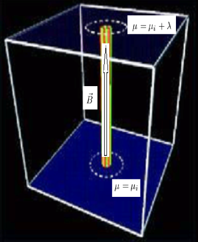
Figure 1: A thin tube surrounding a magnetic field line

the magnetic flux contained within the tube is:

$$\Delta\Phi=\int\vec{B}\cdot d\vec{S}$$ (38)

and the mass contained with the tube is:

$$\Delta M=\int\rho d\vec{l}\cdot d\vec{S},$$ (39)

in which $dl$ is a length element along the tube. Since the magnetic field lines move with the flow by virtue of equation (1) both the quantities $\Delta\Phi$ and $\Delta M$ are conserved and since the tube is thin we may define the conserved magnetic load:

$$\lambda=\frac{\Delta M}{\Delta\Phi}=\oint\frac{\rho}{B}dl,$$ (40)

in which the above integral is performed along the field line. Obviously the parts of the line which go out of the flow to regions in which $\rho=0$ have a null contribution to the integral. Notice that $\lambda$ is a single valued function that can be measured in principle. Since $\lambda$ is conserved it satisfies the equation:

$$\frac{d\lambda}{dt}=0.$$ (41)

By construction surfaces of constant magnetic load move with the flow and contain magnetic field lines. Hence the gradient to such surfaces must be orthogonal to the field line:

$$\vec{\nabla}\lambda\cdot\vec{B}=0.$$ (42)

Now consider an arbitrary comoving point on the magnetic field line and denote it by $i$, and consider an additional comoving point on the magnetic field line and denote it by $r$. The integral:

$$\mu(r)=\int_{i}^{r}\frac{\rho}{B}dl+\mu(i),$$ (43)

is also a conserved quantity which we may denote following Lynden-Bell & Katz [25] as the magnetic metage. $\mu(i)$ is an arbitrary number which can be chosen differently for each magnetic line. By construction:

$$\frac{d\mu}{dt}=0.$$ (44)

Also it is easy to see that by differentiating along the magnetic field line we obtain:

$$\vec{\nabla}\mu\cdot\vec{B}=\rho.$$ (45)

Notice that $\mu$ will be generally a non single valued function, we will show later in this paper that symmetry to translations in $\mu$ will generate through the Noether theorem the conservation of the magnetic cross helicity.

At this point we have two comoving coordinates of flow, namely $\lambda,\mu$ obviously in a three dimensional flow we also have a third coordinate. However, before defining the third coordinate we will find it useful to work not directly with $\lambda$ but with a function of $\lambda$. Now consider the magnetic flux within a surface of constant load $\Phi(\lambda)$ as described in figure 2

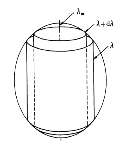
Figure 2: Surfaces of constant load

(the figure was given by Lynden-Bell & Katz [25]). The magnetic flux is a conserved quantity and depends only on the load $\lambda$ of the surrounding surface. Now we define the quantity:

$$\chi=\frac{\Phi(\lambda)}{2\pi}.$$ (46)

Obviously $\chi$ satisfies the equations:

$$\frac{d\chi}{dt}=0,\qquad\vec{B}\cdot\vec{\nabla}\chi=0,$$ (47)

we will immediately show that this function is identical to Sakurai’s function defined in equation (17). Let us now define an additional comoving coordinate $\eta^{*}$ since $\vec{\nabla}\mu$ is not orthogonal to the $\vec{B}$ lines we can choose $\vec{\nabla}\eta^{*}$ to be orthogonal to the $\vec{B}$ lines and not be in the direction of the $\vec{\nabla}\chi$ lines, that is we choose $\eta^{*}$ not to depend only on $\chi$. Since both $\vec{\nabla}\eta^{*}$ and $\vec{\nabla}\chi$ are orthogonal to $\vec{B}$, $\vec{B}$ must take the form:

$$\vec{B}=A\vec{\nabla}\chi\times\vec{\nabla}\eta^{*}.$$ (48)

However, using equation (2) we have:

$$\vec{\nabla}\cdot\vec{B}=\vec{\nabla}A\cdot(\vec{\nabla}\chi\times\vec{\nabla}\eta^{*})=0.$$ (49)

Which implies that $A$ is a function of $\chi,\eta^{*}$. Now we can define a new comoving function $\eta$ such that:

$$\eta=\int_{0}^{\eta^{*}}A(\chi,\eta^{{}^{\prime}*})d\eta^{{}^{\prime}*},\qquad\frac{d\eta}{dt}=0.$$ (50)

In terms of this function we recover the Sakurai presentation defined in equation (17):

$$\vec{B}=\vec{\nabla}\chi\times\vec{\nabla}\eta.$$ (51)

Hence we have shown how $\chi,\eta$ can be constructed for a known $\vec{B},\rho$. Notice however, that $\eta$ is defined in a non unique way since one can redefine $\eta$ for example by performing the following transformation: $\eta\rightarrow\eta+f(\chi)$ in which $f(\chi)$ is an arbitrary function. The comoving coordinates $\chi,\eta$ serve as labels of the magnetic field lines. Moreover the magnetic flux can be calculated as:

$$\Phi=\int\vec{B}\cdot d\vec{S}=\int d\chi d\eta.$$ (52)

In the case that the surface integral is performed inside a load contour we obtain:

$$\Phi(\lambda)=\int_{\lambda}d\chi d\eta=\chi\int_{\lambda}d\eta=\left\{\begin{array}[]{c}\chi[\eta]\\ \chi(\eta_{max}-\eta_{min})\\ \end{array}\right.$$ (53)

Comparing the above equation with equation (46) we derive that $\eta$ can be either single valued or not single valued and that its discontinuity across its cut in the non single valued case is $[\eta]=2\pi$.

We will now show how the potentials $\alpha,\beta,\nu$ can be derived. Let us calculate the vorticity $\vec{\omega}$ of the flow. By taking the curl of equation (27) we obtain:

$$\vec{\omega}\equiv\vec{\nabla}\times\vec{v}=\vec{\nabla}\alpha\times\vec{\nabla}\chi+\vec{\nabla}\beta\times\vec{\nabla}\eta.$$ (54)

The following identities are derived:

$$\vec{\omega}\cdot\vec{\nabla}\chi=(\vec{\nabla}\beta\times\vec{\nabla}\eta)\cdot\vec{\nabla}\chi=-\vec{\nabla}\beta\cdot\vec{B},$$ (55)

$$\vec{\omega}\cdot\vec{\nabla}\eta=(\vec{\nabla}\alpha\times\vec{\nabla}\chi)\cdot\vec{\nabla}\eta=\vec{\nabla}\alpha\cdot\vec{B}.$$ (56)

Now let us perform integrations along $\vec{B}$ lines starting from an arbitrary point denoted as $i$ to another arbitrary point denoted as $r$.

$$\beta(r)=-\int_{i}^{r}\frac{\vec{\omega}\cdot\vec{\nabla}\chi}{B}dl+\beta(i),$$ (57)

$$\alpha(r)=\int_{i}^{r}\frac{\vec{\omega}\cdot\vec{\nabla}\eta}{B}dl+\alpha(i).$$ (58)

The numbers $\alpha(i),\beta(i)$ can be chosen in an arbitrary way for each magnetic field line. Hence we have derived (in a non-unique way) the values of the $\alpha,\beta$ functions. Finally we can use equation (27) to derive the function $\nu$ for any point $s$ within the flow:

$$\nu(s)=\int_{i}^{s}(\vec{v}-\alpha\vec{\nabla}\chi-\beta\vec{\nabla}\eta)\cdot d\vec{r}+\nu(i),$$ (59)

in which $i$ is any arbitrary point within the flow, the result will not depend on the trajectory taken in the case that $\nu$ is single valued. If $\nu$ is not single valued on should introduce a cut which the integration trajectory should not cross.

4.4 Stationary barotropic magnetohydrodynamics

Stationary flows are a unique phenomena of Eulerian fluid dynamics which has no counter part in Lagrangian fluid dynamics. The stationary flow is defined by the fact that the physical fields $\vec{v},\vec{B},\rho$ do not depend on the temporal coordinate. This, however, does not imply that the corresponding potentials $\alpha,\beta,\chi,\eta,\nu$ are all functions of spatial coordinates alone. Moreover, it can be shown that choosing the potentials in such a way will lead to erroneous results in the sense that the stationary equations of motion can not be derived from the Lagrangian density $\hat{\cal L}$ given in equation (37). However, this problem can be amended easily as follows. Let us choose $\alpha,\beta,\chi,\nu$ to depend on the spatial coordinates alone. Let us choose $\eta$ such that:

$$\eta=\bar{\eta}-t,$$ (60)

in which $\bar{\eta}$ is a function of the spatial coordinates. The Lagrangian density $\hat{\cal L}$ given in equation (37) will take the form:

$$\hat{\cal L}=\rho(\beta-\varepsilon(\rho))-\frac{1}{2}\rho(\vec{\nabla}\nu+\alpha\vec{\nabla}\chi+\beta\vec{\nabla}\bar{\eta})^{2}-\frac{1}{8\pi}(\vec{\nabla}\chi\times\vec{\nabla}\bar{\eta})^{2}.$$ (61)

The above functional can be compared with Vladimirov and Moffatt [4] equation 6.12 for incompressible flows in which their $I$ is analogue to our $\beta$. Notice however, that while $\beta$ is not a conserved quantity $I$ is.

Varying the Lagrangian $\hat{L}=\int\hat{\cal L}d^{3}x$ with respect to $\nu,\alpha,\beta,\chi,\eta,\rho$ leads to the following equations:

$$\vec{\nabla}\cdot(\rho\hat{\vec{v}})=0,$$

$$\rho\hat{\vec{v}}\cdot\vec{\nabla}\chi=0,$$

$$\rho(\hat{\vec{v}}\cdot\vec{\nabla}\bar{\eta}-1)=0,$$

$$\hat{\vec{v}}\cdot\vec{\nabla}\alpha=\frac{\vec{\nabla}\bar{\eta}\cdot\hat{\vec{J}}}{\rho},\qquad$$

$$\hat{\vec{v}}\cdot\vec{\nabla}\beta=-\frac{\vec{\nabla}\chi\cdot\hat{\vec{J}}}{\rho},$$

$$\beta=\frac{1}{2}\hat{\vec{v}}^{2}+w.$$ (62)

Calculations similar to the ones done in previous subsections will show that those equations lead to the stationary barotropic magnetohydrodynamic equations:

$$\vec{\nabla}\times(\hat{\vec{v}}\times\hat{\vec{B}})=0,$$ (63)

$$\rho(\hat{\vec{v}}\cdot\vec{\nabla})\hat{\vec{v}}=-\vec{\nabla}p(\rho)+\frac{(\vec{\nabla}\times\hat{\vec{B}})\times\hat{\vec{B}}}{4\pi}.$$ (64)

5 The Simplified Hamiltonian Formalism

Let us derive the conjugate momenta of the variables appearing in the Lagrangian density $\hat{\cal L}$ defined in equation (37). A simple calculation will yield:

$$\pi_{\nu}\equiv\frac{\partial\hat{\cal L}}{\partial\left(\frac{\partial{\nu}}{\partial t}\right)}=-\rho,\quad\pi_{\chi}\equiv\frac{\partial\hat{\cal L}}{\partial\left(\frac{\partial{\chi}}{\partial t}\right)}=-\rho\alpha,\quad\pi_{\eta}\equiv\frac{\partial\hat{\cal L}}{\partial\left(\frac{\partial{\eta}}{\partial t}\right)}=-\rho\beta.$$ (65)

The rest of the canonical momenta $\pi_{\rho},\pi_{\alpha},\pi_{\beta}$ are null. It thus seems that the six functions appearing in the Lagrangian density $\hat{\cal L}$ can be divided to ”approximate” conjugate pairs: $(\nu,\rho),(\chi,\alpha),(\eta,\beta)$. The Hamiltonian density $\hat{\cal H}$ can be now calculated as follows:

$$\hat{\cal H}=\pi_{\nu}\frac{\partial{\nu}}{\partial t}+\pi_{\chi}\frac{\partial{\chi}}{\partial t}+\pi_{\eta}\frac{\partial{\eta}}{\partial t}-\hat{\cal L}=\rho\left[\varepsilon(\rho)+\frac{1}{2}\hat{\vec{v}}^{2}\right]+\frac{1}{8\pi}\hat{\vec{B}}^{2},$$ (66)

in which $\hat{\vec{v}}$ is defined in equation (27) and $\hat{\vec{B}}$ is defined in equation (25). This Hamiltonian was previously introduced by Frenkel, Levich & Stilman [2] using somewhat different variables. The equations derived from the above Hamiltonian density are similar to equations (24), equation (29) and equations (32) and will not be re-derived here. While Frenkel, Levich & Stilman [2] have postulated the Hamiltonian density appearing in equation (66), this Hamiltonian is here derived from a Lagrangian.

6 Simplified variational principle of stationary barotropic magnetohydrodynamics

In the previous section we have shown that barotropic magnetohydrodynamics can be described in terms of six first order differential equations or of an action principle from which those equations can be derived. This formalism was shown to apply to both stationary and non-stationary magnetohydrodynamics. Although for non-stationary magnetohydrodynamics we do not know at present how the number of functions can be further reduced, for stationary barotropic magnetohydrodynamics the situation is quite different. In fact we will show that for stationary barotropic magnetohydrodynamics three functions will suffice.

Consider equation (47), for a stationary flow it takes the form:

$$\vec{v}\cdot\vec{\nabla}\chi=0.$$ (67)

Hence $\vec{v}$ can take the form:

$$\vec{v}=\frac{\vec{\nabla}\chi\times\vec{K}}{\rho}.$$ (68)

However, since the velocity field must satisfy the stationary mass conservation equation (3):

$$\vec{\nabla}\cdot(\rho\vec{v})=0.$$ (69)

We see that $\vec{K}$ must have the form $\vec{K}=\vec{\nabla}N$, where $N$ is an arbitrary function. Thus, $\vec{v}$ takes the form:

$$\vec{v}=\frac{\vec{\nabla}\chi\times\vec{\nabla}N}{\rho}.$$ (70)

Let us now calculate $\vec{v}\times\vec{B}$ in which $\vec{B}$ is given by Sakurai’s presentation equation (25):

$$\vec{v}\times\vec{B} = (\frac{\vec{\nabla}\chi\times\vec{\nabla}N}{\rho})\times(\vec{\nabla}\chi\times\vec{\nabla}\eta)$$ (71)

$$= \frac{1}{\rho}\vec{\nabla}\chi(\vec{\nabla}\chi\times\vec{\nabla}N)\cdot\vec{\nabla}\eta.$$

Since the flow is stationary $N$ can be at most a function of the three comoving coordinates $\chi,\mu,\bar{\eta}$ defined in subsections 4.3 and 4.4, hence:

$$\vec{\nabla}N=\frac{\partial N}{\partial\chi}\vec{\nabla}\chi+\frac{\partial N}{\partial\mu}\vec{\nabla}\mu+\frac{\partial N}{\partial\bar{\eta}}\vec{\nabla}\bar{\eta}.$$ (72)

Inserting equation (72) into equation (71) will yield:

$$\vec{v}\times\vec{B}=\frac{1}{\rho}\vec{\nabla}\chi\frac{\partial N}{\partial\mu}(\vec{\nabla}\chi\times\vec{\nabla}\mu)\cdot\vec{\nabla}\bar{\eta}.$$ (73)

Rearranging terms and using Sakurai’s presentation equation (25) we can simplify the above equation and obtain:

$$\vec{v}\times\vec{B}=-\frac{1}{\rho}\vec{\nabla}\chi\frac{\partial N}{\partial\mu}(\vec{\nabla}\mu\cdot\vec{B}).$$ (74)

However, using equation (44) this will simplify to the form:

$$\vec{v}\times\vec{B}=-\vec{\nabla}\chi\frac{\partial N}{\partial\mu}.$$ (75)

Now let us consider equation (1); for stationary flows this will take the form:

$$\vec{\nabla}\times(\vec{v}\times\vec{B})=0.$$ (76)

Inserting equation (74) into equation (63) will lead to the equation:

$$\vec{\nabla}(\frac{\partial N}{\partial\mu})\times\vec{\nabla}\chi=0.$$ (77)

However, since $N$ is at most a function of $\chi,\mu,\bar{\eta}$ it follows that $\frac{\partial N}{\partial\mu}$ is some function of $\chi$:

$$\frac{\partial N}{\partial\mu}=-F(\chi).$$ (78)

This can be easily integrated to yield:

$$N=-\mu F(\chi)+G(\chi,\bar{\eta}).$$ (79)

Inserting this back into equation (70) will yield:

$$\vec{v}=\frac{\vec{\nabla}\chi\times(-F(\chi)\vec{\nabla}\mu+\frac{\partial G}{\partial\bar{\eta}}\vec{\nabla}\bar{\eta})}{\rho}.$$ (80)

Let us now replace the set of variables $\chi,\bar{\eta}$ with a new set $\chi^{\prime},\bar{\eta}^{\prime}$ such that:

$$\chi^{\prime}=\int F(\chi)d\chi,\qquad\bar{\eta}^{\prime}=\frac{\bar{\eta}}{F(\chi)}.$$ (81)

This will not have any effect on the Sakurai representation given in equation (25) since:

$$\vec{B}=\vec{\nabla}\chi\times\vec{\nabla}\eta=\vec{\nabla}\chi\times\vec{\nabla}\bar{\eta}=\vec{\nabla}\chi^{\prime}\times\vec{\nabla}\bar{\eta}^{\prime}.$$ (82)

However, the velocity will have a simpler representation and will take the form:

$$\vec{v}=\frac{\vec{\nabla}\chi^{\prime}\times\vec{\nabla}(-\mu+G^{\prime}(\chi^{\prime},\bar{\eta}^{\prime}))}{\rho},$$ (83)

in which $G^{\prime}=\frac{G}{F}$. At this point one should remember that $\mu$ was defined in equation (43) up to an arbitrary constant which can vary between magnetic field lines. Since the lines are labelled by their $\chi^{\prime},\bar{\eta}^{\prime}$ values it follows that we can add an arbitrary function of $\chi^{\prime},\bar{\eta}^{\prime}$ to $\mu$ without effecting its properties. Hence we can define a new $\mu^{\prime}$ such that:

$$\mu^{\prime}=\mu-G^{\prime}(\chi^{\prime},\bar{\eta}^{\prime}).$$ (84)

Notice that $\mu^{\prime}$ can be multi-valued; this will be discussed in somewhat more detail in subsection 6.3. Inserting equation (84) into equation (83) will lead to a simplified equation for $\vec{v}$:

$$\vec{v}=\frac{\vec{\nabla}\mu^{\prime}\times\vec{\nabla}\chi^{\prime}}{\rho}.$$ (85)

In the following the primes on $\chi,\mu,\bar{\eta}$ will be ignored. The above equation is analogues to Vladimirov and Moffatt’s [4] equation 7.11 for incompressible flows, in which our $\mu$ and $\chi$ play the part of their $A$ and $\Psi$. It is obvious that $\vec{v}$ satisfies the following set of equations:

$$\vec{v}\cdot\vec{\nabla}\mu=0,\qquad\vec{v}\cdot\vec{\nabla}\chi=0,\qquad\vec{v}\cdot\vec{\nabla}\bar{\eta}=1,$$ (86)

to derive the right hand equation we have used both equation (44) and equation (25). Hence $\mu,\chi$ are both comoving and stationary. As for $\bar{\eta}$ it satisfies the same equation as $\bar{\eta}$ defined in equation (60) as can be seen from equation (62). It can be easily seen that if:

$$basis=(\vec{\nabla}\chi,\vec{\nabla}\bar{\eta},\vec{\nabla}\mu),$$ (87)

is a local vector basis at any point in space than their exists a dual basis:

$$dual\ basis=\frac{1}{\rho}(\vec{\nabla}\bar{\eta}\times\vec{\nabla}\mu,\vec{\nabla}\mu\times\vec{\nabla}\chi,\vec{\nabla}\chi\times\vec{\nabla}\bar{\eta})=(\frac{\vec{\nabla}\bar{\eta}\times\vec{\nabla}\mu}{\rho},\vec{v},\frac{\vec{B}}{\rho}).$$ (88)

Such that:

$$basis_{i}\cdot dual\ basis_{j}=\delta_{ij},\qquad i,j\in[1,2,3],$$ (89)

in which $\delta_{ij}$ is Kronecker’s delta. Hence while the surfaces $\chi,\mu,\bar{\eta}$ generate a local vector basis for space, the physical fields of interest $\vec{v},\vec{B}$ are part of the dual basis. By vector multiplying $\vec{v}$ and $\vec{B}$ and using equations (85,25) we obtain:

$$\vec{v}\times\vec{B}=\vec{\nabla}\chi,$$ (90)

this means that both $\vec{v}$ and $\vec{B}$ lie on $\chi$ surfaces and provide a vector basis for this two dimensional surface. The above equation can be compared with Vladimirov and Moffatt [4] equation 5.6 for incompressible flows in which their $J$ is analogue to our $\chi$.

6.1 The action principle

In the previous subsection we have shown that if the velocity field $\vec{v}$ is given by equation (85) and the magnetic field $\vec{B}$ is given by the Sakurai representation equation (25) than equations (1,2,3) are satisfied automatically for stationary flows. To complete the set of equations we will show how the Euler equations (4) can be derived from the action given in equation (6) in which both $\vec{v}$ and $\vec{B}$ are given by equation (85) and equation (25) respectively and the density $\rho$ is given by equation (44):

$$\rho=\vec{\nabla}\mu\cdot\vec{B}=\vec{\nabla}\mu\cdot(\vec{\nabla}\chi\times\vec{\nabla}\eta)=\frac{\partial(\chi,\eta,\mu)}{\partial(x,y,z)}.$$ (91)

In this case the Lagrangian density of equation (6) will take the form:

$${\cal L}=\rho(\frac{1}{2}(\frac{\vec{\nabla}\mu\times\vec{\nabla}\chi}{\rho})^{2}-\varepsilon(\rho))-\frac{(\vec{\nabla}\chi\times\vec{\nabla}\eta)^{2}}{8\pi}$$ (92)

and can be seen explicitly to depend on only three functions. Let us make arbitrary small variations $\delta\alpha_{i}=(\delta\chi,\delta\eta,\delta\mu)$ of the functions $\alpha_{i}=(\chi,\eta,\mu)$. Let us define the vector:

$$\vec{\xi}\equiv-\frac{\partial\vec{r}}{\partial\alpha_{i}}\delta\alpha_{i}.$$ (93)

This will lead to the equation:

$$\delta\alpha_{i}=-\vec{\nabla}\alpha_{i}\cdot\vec{\xi}.$$ (94)

And by virtue of equation (10) we have:

$$\Delta\alpha_{i}=\delta\alpha_{i}+(\vec{\xi}\cdot\vec{\nabla})\alpha_{i}=0,$$ (95)

as one should expect since $\alpha_{i}$ are comoving with the flow. Making a variation of $\rho$ given in equation (91) with respect to $\alpha_{i}$ will yield equation (8). Furthermore, taking the variation of $\vec{B}$ given by Sakurai’s representation (25) with respect to $\alpha_{i}$ will yield equation (9). It remains to calculate $\delta\vec{v}$ by varying equation (85) this will yield:

$$\delta\vec{v}=-\frac{\delta\rho}{\rho}\vec{v}+\frac{1}{\rho}\vec{\nabla}\times(\rho\vec{\xi}\times\vec{v}).$$ (96)

Inserting equations (8,9,96) into equation (7) will yield:

$$\delta{\cal L} = \vec{v}\cdot\vec{\nabla}\times(\rho\vec{\xi}\times\vec{v})-\frac{\vec{B}\cdot\vec{\nabla}\times(\vec{\xi}\times\vec{B})}{4\pi}-\delta\rho(\frac{1}{2}\vec{v}^{2}+w)$$ (97)

$$= \vec{v}\cdot\vec{\nabla}\times(\rho\vec{\xi}\times\vec{v})-\frac{\vec{B}\cdot\vec{\nabla}\times(\vec{\xi}\times\vec{B})}{4\pi}+\vec{\nabla}\cdot(\rho\vec{\xi})(\frac{1}{2}\vec{v}^{2}+w).$$

Using the well known vector identity:

$$\vec{A}\cdot\vec{\nabla}\times(\vec{C}\times\vec{A})=\vec{\nabla}\cdot((\vec{C}\times\vec{A})\times\vec{A})+(\vec{C}\times\vec{A})\cdot\vec{\nabla}\times\vec{A}$$ (98)

and the theorem of Gauss we can write now equation (7) in the form:

$$\delta A = \int dt\{\oint d\vec{S}\cdot[\rho(\vec{\xi}\times\vec{v})\times\vec{v}-\frac{(\vec{\xi}\times\vec{B})\times\vec{B}}{4\pi}+(\frac{1}{2}\vec{v}^{2}+w)\rho\vec{\xi}]$$ (99)

$$+ \int d^{3}x\vec{\xi}\cdot[\rho\vec{v}\times\vec{\omega}+\vec{J}\times\vec{B}-\rho\vec{\nabla}(\frac{1}{2}\vec{v}^{2}+w)]\}.$$

The time integration is of course redundant in the above expression. Also notice that we have used the current definition equation (5) and the vorticity definition equation (54). Suppose now that $\delta A=0$ for a $\vec{\xi}$ such that the boundary term (including both the boundary of the domain and relevant cuts) in the above equation is null but that $\vec{\xi}$ is otherwise arbitrary, then it entails the equation:

$$\rho\vec{v}\times\vec{\omega}+\vec{J}\times\vec{B}-\rho\vec{\nabla}(\frac{1}{2}\vec{v}^{2}+w)=0.$$ (100)

Using the well known vector identity:

$$\frac{1}{2}\vec{\nabla}(\vec{v}^{2})=(\vec{v}\cdot\vec{\nabla})\vec{v}+\vec{v}\times(\vec{\nabla}\times\vec{v})$$ (101)

and rearranging terms we recover the stationary Euler equation:

$$\rho(\vec{v}\cdot\vec{\nabla})\vec{v}=-\vec{\nabla}p+\vec{J}\times\vec{B}.$$ (102)

6.2 The case of an axi-symmetric magnetic field

Consider an axi-symmetric magnetic field such that the magnetic field is dependent only on the coordinate $R$ which is the distance from the axis of symmetry and the coordinate $z$ which is the distance along the axis of symmetry from an arbitrary origin on the axis. Thus:

$$\vec{B}=\vec{B}(R,z).$$ (103)

Any axi-symmetric magnetic field satisfying equation (2) can be represented in the form:

$$\vec{B}=\vec{\nabla}P\times\vec{\nabla}(\frac{\phi}{2\pi})+2\pi RB_{\phi}\vec{\nabla}(\frac{\phi}{2\pi}).$$ (104)

In which $\phi$ is the azimuthal angle defined in the conventional way and $B_{\phi}$ is the component of $\vec{B}$ in the $\phi$ direction. The function $P=P(R,z)$ is the flux through a circle of radius $R$ at height $z$:

$$P(R,z)=\int_{(R,z)}\vec{B}\cdot d\vec{S}=2\pi\int_{0}^{R}B_{z}(R^{\prime},z)R^{\prime}dR^{\prime}.$$ (105)

For finite field configurations $P$ will have a maximum $P_{m}=P(R_{m},z_{m})$ at some $R_{m},z_{m}$. This circle $R=R_{m}$ will form a line toroid with the other constant $P$ surfaces nearby forming a nested set. There can be several such local maxima with local nested toroids in a general configuration but the simpler case has just one.

Let us study the relations between the functions $P,B_{\phi}$ and the functions $\chi,\eta$ given in equation (17). Assuming that the density $\rho$ is axi-symmetric one can see the magnetic load defined in equation (40) is also axi-symmetric and that the surfaces of constant load are surfaces of revolution around the axis of symmetry. From equation (46) we deduce that $\chi=\chi(R,z)$. Expressing equation (17) in terms of the coordinates $R,\phi,z$ results in:

$$\vec{B}=(-\frac{1}{R}\partial_{z}\chi\partial_{\phi}\eta)\hat{R}+(\partial_{z}\chi\partial_{R}\eta-\partial_{R}\chi\partial_{z}\eta)\hat{\phi}+(\frac{1}{R}\partial_{R}\chi\partial_{\phi}\eta)\hat{z}.$$ (106)

In which $\partial_{y}$ is a short hand notation for $\frac{\partial}{\partial y}$ and $\hat{y}$ is a unit vector perpendicular to the constant $y$ surface. Comparing equation (106) with equation (104) we arrive with the set of equations:

$$\partial_{z}P=\partial_{z}\chi\partial_{\phi}(2\pi\eta),\qquad\partial_{R}P=\partial_{R}\chi\partial_{\phi}(2\pi\eta).$$ (107)

From which we derive the equation:

$$\partial_{z}P\partial_{R}\chi-\partial_{R}P\partial_{z}\chi=0\Rightarrow\vec{\nabla}P\times\vec{\nabla}\chi=0.$$ (108)

Hence:

$$P=F(\chi),$$ (109)

where $F$ is an arbitrary function. We deduce that $P$ is just another type of labelling of the load surfaces. Thus equation (107) will lead to:

$$\partial_{\phi}(2\pi\eta)=\frac{dP}{d\chi}\Rightarrow\eta=\frac{\phi}{2\pi}\frac{dP}{d\chi}+\tilde{\eta}(R,z).$$ (110)

This should be compared with the result of Young et al. [9, equation 5.1]. Substituting the above result in equation (106) will lead to the equation:

$$B_{\phi}\hat{\phi}=(\partial_{z}\chi\partial_{R}\tilde{\eta}-\partial_{R}\chi\partial_{z}\tilde{\eta})\hat{\phi}=\vec{\nabla}\chi\times\vec{\nabla}\tilde{\eta}.$$ (111)

This can also be written as:

$$B_{\phi}=\hat{\phi}\cdot(\vec{\nabla}\chi\times\vec{\nabla}\tilde{\eta})=(\hat{\phi}\times\vec{\nabla}\chi)\cdot\vec{\nabla}\tilde{\eta}.$$ (112)

Hence $B_{\phi}$ is proportional to the gradient of $\tilde{\eta}$ along the $\hat{\phi}\times\vec{\nabla}\chi$ direction. Since $\hat{\phi}\times\vec{\nabla}\chi$ is known we can integrate along this vector to obtain a non-unique solution for $\tilde{\eta}$:

$$\tilde{\eta}=\int\frac{B_{\phi}}{|\hat{\phi}\times\vec{\nabla}\chi|}dl,$$ (113)

in which $dl$ is a line element along the $\hat{\phi}\times\vec{\nabla}\chi$ line.

6.3 The case of a magnetic field on a toroid

Our previous definitions of the surfaces of constant load given in equation (40) is ambiguous when the field lines are ”surface filling” eg on a toroid and give no result when the field lines are ”volume filling”. At equilibrium $\vec{B}$ and $\vec{v}$ lie in surfaces (there is an exception when $\vec{B}$ and $\vec{v}$ are parallel and fill volumes). Our former considerations apply unchanged if these surfaces have the topology of cylinders but they need generalization when the surfaces have the topology of toroids nested on a line (a similar discussion in which non-magnetic fluids are considered can be found in [23]). We consider a surface $\Sigma$ spanning that line toroid. Each toroid $T$ will meet $\Sigma$ in a loop. Consider the magnetic flux $\Phi(T)$ through that part of $\Sigma$ within the loop and the mass enclosed by the toroid $m(T)$. The the mass outside the toroid is $\tilde{m}(T)=M-m(T)$. Now express $\tilde{m}$ as a function $\tilde{m}(\Phi)$ of the magnetic flux $\Phi$, then a definition of magnetic load analogous to that for ”cylinders” parallel to the axis is:

$$\lambda=\frac{d\tilde{m}}{d\Phi}.$$ (114)

However, there are now two loads corresponding to the two fluxes associated with a given toroid. The other load is obtained by taking a cut across the ”short” circle section of the torus say of constant $\phi$. The magnetic flux $\Phi^{*}$ through such a cross section may be expressed as a function of the total mass $m(T)$ within the toroid and

$$\lambda^{*}=\frac{dm}{d\Phi^{*}},$$ (115)

is a second different load. Of course it is also permissible to reexpress the flux $\Phi^{*}$ as a function of the flux $\Phi$ then we find:

$$\lambda^{*}=\frac{dm}{d\Phi^{*}}=\frac{\frac{dm}{d\Phi}}{\frac{d\Phi^{*}}{d\Phi}}=-\frac{\lambda}{\frac{d\Phi^{*}}{d\Phi}}.$$ (116)

The surfaces of constant $\lambda$ are of course the toroids $T$ which also have $\lambda^{*}$ constant.

A similar problem may arise with the definition of the magnetic metage defined in equation (43). We may wish to define this quantity using the magnetic field $\vec{B}$ and velocity field $\vec{v}$. Since those vectors provide a vector basis on the load surface, they can be combined in such a way say: $\vec{B}+\gamma(\chi)\vec{v}$ to create a vector which is directed along the large loop of the toroid. (A different $\gamma$ will leave only twists around the short way.) This combination represents an unwinding of the field lines so that they no longer twist around the short (long) way. Those loops can be thought as composing the surface $\Sigma$. Another surface $\Sigma^{\prime}$ also composed of such untwisted loops can be so chosen that the mass between $\Sigma$ and $\Sigma^{\prime}$ and between loads $\lambda$ and $\lambda+d\lambda$ is some fixed fraction of $\frac{dm}{d\lambda}d\lambda$. Such $\Sigma^{\prime}$ form suitable constant metage surfaces $\mu$ corresponding to partial loads $\lambda$. Notice that $2\pi\mu$ then describes the angle from $\Sigma$ turned around the toroid by the short way to reach any chosen point. Similar use of the other load $\lambda^{*}$ allows us to define another generalized angle $\mu^{*}$ measured around the long way. A somewhat less physical approach is given below.

Let us consider a toroid of constant magnetic load. Dungey [19, p. 31] has considered the case in which magnetic field lines lie on a torus. He has shown that one of the functions (ie $\eta$) involved in the representation (17) should be non-single valued and therefore a cut should be introduced.

In order to obtain a simple looking cuts we will replace the previous set of functions $\mu,\eta$ with a new set $\phi^{*},\eta^{*}$, which will be defined as follows:

$$\phi^{*} \equiv \frac{\mu+G(\chi)\eta}{\Omega(\chi)},$$

$$\eta^{*} \equiv \frac{\eta-\phi^{*}}{f(\chi)},$$ (117)

$G,\Omega,f$ are arbitrary functions of $\chi$. Therefore $\mu$ and $\eta$ can be given in terms of $\phi^{*},\eta^{*}$ as:

$$\eta = \phi^{*}+f(\chi)\eta^{*},$$

$$\mu = -G(\chi)\eta+\Omega(\chi)\phi^{*},$$ (118)

$\eta^{*}$ can be considered as an angle varying over the small circle of the torus, while $\phi^{*}$ can be considered as an angle varying over the large circle of the torus as in figure (3). On the torus of constant magnetic load the $\phi^{*},\eta^{*}$ functions have a simple ”cut” structure.

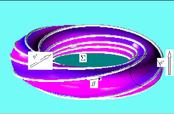
Figure 3: A torus of magnetic field lines

The above equation can also serve as a ”definition” of $\mu$. Inserting equations (118) into equation (17) and equation (85) will result in the following set of equations:

$$\vec{B} = \vec{\nabla}\chi\times\vec{\nabla}\phi^{*}+f(\chi)\vec{\nabla}\chi\times\vec{\nabla}\eta^{*},$$

$$\vec{v} = G(\chi)\frac{\vec{B}}{\rho}+\Omega(\chi)\frac{\vec{\nabla}\phi^{*}\times\vec{\nabla}\chi}{\rho}.$$ (119)

Hence $\vec{B}$ is partitioned into two vectors circulating along the small and large circles of the torus. While $\vec{v}$ has two vector components one along the magnetic field $\vec{B}$ and another along the small circle.

7 Topological constants of motion

Magnetohydrodynamics is known to have the following two topological constants of motion; one is the magnetic helicity:

$${\cal H}_{M}\equiv\int\vec{B}\cdot\vec{A}d^{3}x,$$ (120)

which is known to measure the degree of knottiness of lines of the magnetic field $\vec{B}$ [26]. In the above equation $\vec{A}$ is the vector potential defined implicitly by the equation:

$$\vec{B}=\vec{\nabla}\times\vec{A}.$$ (121)

The other topological constant is the magnetic cross helicity:

$${\cal H}_{C}\equiv\int\vec{B}\cdot\vec{v}d^{3}x,$$ (122)

characterizing the degree of cross knottiness of the magnetic field and velocity lines.

7.1 Representation in terms of the magnetohydrodynamic potentials

Let us write the topological constants given in equation (120) and equation (122) in terms of the magnetohydrodynamic potentials $\alpha,\beta,\chi,\eta,\nu,\rho$ introduced in previous sections.

First let us combine equation (17) with equation (121) to obtain the equation:

$$\vec{\nabla}\times(\vec{A}-\chi\vec{\nabla}\eta)=0,$$ (123)

this leads immediately to the result:

$$\vec{A}=\chi\vec{\nabla}\eta+\vec{\nabla}\zeta,$$ (124)

in which $\zeta$ is some function. Let us now calculate the scalar product $\vec{B}\cdot\vec{A}$:

$$\vec{B}\cdot\vec{A}=(\vec{\nabla}\chi\times\vec{\nabla}\eta)\cdot\vec{\nabla}\zeta.$$ (125)

However, since we have the local vector basis: $(\vec{\nabla}\chi,\vec{\nabla}\eta,\vec{\nabla}\mu)$ we can write $\vec{\nabla}\zeta$ as:

$$\vec{\nabla}\zeta=\frac{\partial\zeta}{\partial\chi}\vec{\nabla}\chi+\frac{\partial\zeta}{\partial\mu}\vec{\nabla}\mu+\frac{\partial\zeta}{\partial\eta}\vec{\nabla}\eta.$$ (126)

Hence we can write:

$$\vec{B}\cdot\vec{A}=\frac{\partial\zeta}{\partial\mu}(\vec{\nabla}\chi\times\vec{\nabla}\eta)\cdot\vec{\nabla}\mu=\frac{\partial\zeta}{\partial\mu}\frac{\partial(\chi,\eta,\mu)}{\partial(x,y,z)}.$$ (127)

Now we can insert equation (127) into equation (120) to obtain the expression:

$${\cal H}_{M}=\int\frac{\partial\zeta}{\partial\mu}d\mu d\chi d\eta.$$ (128)

We can think about the magnetohydrodynamic domain as composed of thin closed tubes of magnetic lines each labelled by $(\chi,\eta)$. Performing the integration along such a thin tube in the metage direction results in:

$$\oint_{\chi,\eta}\frac{\partial\zeta}{\partial\mu}d\mu=[\zeta]_{\chi,\eta},$$ (129)

in which $[\zeta]_{\chi,\eta}$ is the discontinuity of the function $\zeta$ along its cut. Thus a thin tube of magnetic lines in which $\zeta$ is single valued does not contribute to the magnetic helicity integral. Inserting equation (129) into equation (140) will result in:

$${\cal H}_{M}=\int[\zeta]_{\chi,\eta}d\chi d\eta=\int[\zeta]d\Phi,$$ (130)

in which we have used equation (52). Hence:

$$[\zeta]=\frac{d{\cal H}_{M}}{d\Phi},$$ (131)

the discontinuity of $\zeta$ is thus the density of magnetic helicity per unit of magnetic flux in a tube. We deduce that the Sakurai representation does not entail zero magnetic helicity, rather it is perfectly consistent with non zero magnetic helicity as was demonstrated above and in agreement to the claims made by Frenkel, Levich & Stilman [2]. Notice however, that the topological structure of the magnetohydrodynamic flow constrain the gauge freedom which is usually attributed to vector potential $\vec{A}$ and limits it to single valued functions. Moreover, while the choice of $\vec{A}$ is arbitrary since one can add to $\vec{A}$ an arbitrary gradient of a single valued function which may lead to different choices of $\zeta$ the discontinuity value $[\zeta]$ is not arbitrary and has a physical meaning given above.

Let us now introduce the velocity expression given in equation (27) and calculate the scalar product of $\vec{B}$ and $\vec{v}$, using the same arguments as in the previous paragraph will lead to the expression:

$$\vec{v}\cdot\vec{B}=\frac{\partial\nu}{\partial\mu}(\vec{\nabla}\chi\times\vec{\nabla}\eta)\cdot\vec{\nabla}\mu=\frac{\partial\nu}{\partial\mu}\frac{\partial(\chi,\eta,\mu)}{\partial(x,y,z)}.$$ (132)

Inserting equation (132) into equation (122) will result in:

$${\cal H}_{C}=\int\frac{\partial\nu}{\partial\mu}d\mu d\chi d\eta.$$ (133)

We can think about the magnetohydrodynamic domain as composed of thin closed tubes of magnetic lines each labelled by $(\chi,\eta)$. Performing the integration along such a thin tube in the metage direction results in:

$$\oint_{\chi,\eta}\frac{\partial\nu}{\partial\mu}d\mu=[\nu]_{\chi,\eta},$$ (134)

in which $[\nu]_{\chi,\eta}$ is the discontinuity of the function $\nu$ along its cut. Thus a thin tube of magnetic lines in which $\nu$ is single valued does not contribute to the cross helicity integral. Inserting equation (134) into equation (133) will result in:

$${\cal H}_{C}=\int[\nu]_{\chi,\eta}d\chi d\eta=\int[\nu]d\Phi,$$ (135)

in which we have used equation (52). Hence:

$$[\nu]=\frac{d{\cal H}_{C}}{d\Phi},$$ (136)

the discontinuity of $\nu$ is thus the density of cross helicity per unit of magnetic flux. We deduce that a flow with null cross helicity will have a single valued $\nu$ function alternatively, a non single valued $\nu$ will entail a non zero cross helicity. Furthermore, from equation (29) it is obvious that:

$$\frac{d[\nu]}{dt}=0.$$ (137)

We conclude that not only is the magnetic cross helicity conserved as an integral quantity of the entire magnetohydrodynamic domain but also the (local) density of cross helicity per unit of magnetic flux is a conserved quantity as well.

In the following sub section we give a simple example which will demonstrate some of the general assertions of this paragraph.

7.2 A Helical Stratified Magnetic Field

Consider a magnetohydrodynamic flow of uniform density $\rho$. Furthermore assume that the flow contains a helical stratified magnetic field:

$$\vec{B}=\left\{\begin{array}[]{ll}2B_{\bot}(1-\frac{R}{a})\hat{\phi}+B_{z0}\hat{z}&R<a\\ 0&R>a\\ \end{array}\right.$$ (138)

in which $R,\phi,z$ are the standard cylindrical coordinates, $\hat{R},\hat{\phi},\hat{z}$ are the corresponding unit vectors and $B_{z0},B_{\bot}$ are constants. The magnetic field is contained in a cylinder of Radius $a$ and is independent of $z$. A possible choice of the vector potential $\vec{A}$ is:

$$\vec{A}=\left\{\begin{array}[]{ll}B_{z0}x\hat{y}+B_{\bot}a(1-\frac{R}{a})^{2}\hat{z},&R<a\\ 0&R>a\\ \end{array}\right.$$ (139)

in which $\hat{y}$ is a unit vector in the $y$ direction. Let us calculate the magnetic helicity of the field using equation (120) . In order to obtain a finite magnetic helicity we assume that the field is contained between the planes $z=0$ and $z=1$ furthermore we assume that the planes $z=0$ and $z=1$ can be identified such that the magnetic field lines are closed. Thus the domain becomes a topological torus. Inserting equation (138) and equation (139) into equation (120) will result in:

$${\cal H}_{M}\equiv\int\vec{B}\cdot\vec{A}d^{3}x=\frac{\pi}{3}a^{3}B_{z0}B_{\bot}$$ (140)

First let us calculate to load using equation (40) (we assume that $R<a$ in the following calculations) we obtain:

$$\lambda=\rho\frac{4\pi B_{\bot}(1-\frac{R}{a})R+B_{z0}}{B_{z0}^{2}+4B_{\bot}^{2}(1-\frac{R}{a})^{2}}=\lambda(R),$$ (141)

hence the load surfaces are cylinders. The $\chi$ function can now be calculated according to equation (46) to yield the value:

$$\chi=\frac{1}{2}B_{z0}R^{2}.$$ (142)

Solving equation (51) for $\eta$ we obtain the following non unique solution:

$$\eta=\frac{2B_{\bot}}{B_{z0}}(1-\frac{R}{a})\frac{z}{a}+\phi.$$ (143)

Substituting equation (142), equation (143) and equation (139) into equation (124) we can solve for $\zeta$ and obtain:

$$\zeta=B_{\bot}z(a-R)+\frac{1}{2}B_{z0}xy.$$ (144)

Since we have identified the $z=0$ and $z=1$ planes the $z$ coordinate is not single valued and therefore $\zeta$ is a non single valued function which has a discontinuity value:

$$[\zeta]=B_{\bot}(a-R).$$ (145)

Thus we can calculate the magnetic helicity using equation (130) and obtain:

$${\cal H}_{M}=\int[\zeta]d\Phi=\frac{\pi}{3}a^{3}B_{z0}B_{\bot},$$ (146)

which coincides with the result of equation (140).

7.3 Cross Helicity Conservation via the Noether Theorem

The conservation of helicity $\int\vec{v}\cdot\vec{\omega}d^{3}x$ in ideal (non-magnetic) barotropic fluid when certain conditions are satisfied in particular, when $\vec{\omega}\cdot\vec{n}=0$ on the (Lagrangian) surface bounding the volume of integration was discovered by Moffat [26]. Moreau [27] has discussed the conservation of helicity from the group theoretical point of view. In his paper he used an enlarged Arnold symmetry group [28] of fluid element labelling to generate the conservation of helicity. Yahalom [30, 31] has shown that the symmetry group generating conservation of helicity becomes a very simple one parameter translation group in the space of labels (alpha space) when represented by Lynden-Bell and Katz [25] labelling. We will now show that in the case of magnetohydrodynamics the same one parameter translation group will generate the magnetic cross helicity via the Noether Theorem.

Let us denote the initial position of a fluid element by $(x^{k}_{0})$, by mass conservation:

$$\rho(x^{k})d^{3}x=\rho(x^{k}_{0})d^{3}x_{0}=\rho(x^{k}_{0}){\partial(x^{1}_{0},x^{2}_{0},x^{3}_{0})\over\partial(\alpha^{1},\alpha^{2},\alpha^{3})}d^{3}\alpha.$$ (147)

Since the initial position of a fluid element can not depend on time it must depend on the label only, and therefore by an appropriate choice of the $\alpha^{\prime}s$ we obtain:

$$\rho(x^{k})d^{3}x=d^{3}\alpha,\qquad\rho={\partial(\alpha^{1},\alpha^{2},\alpha^{3})\over\partial(x^{1},x^{2},x^{3})}.$$ (148)

Where we assume that the above expressions of course exist. Let us look at the action $A$ defined in equation (6).

From the discussion following equation (15) we know that if the $\vec{\xi}$ variations disappear at times ${t_{0}},{t_{1}}$ than A is extremal only if Euler’s equations are satisfied and the boundary term disappears. If on the other hand we make a symmetry displacement i.e. a displacement that makes $\delta A$ vanish and assume that Euler’s equations are satisfied and the boundary term disappears, we obtain that:

$$\int_{V}\vec{v}\cdot\vec{\xi}d^{3}\alpha=const.$$ (149)

this is Noether’s theorem in it’s fluid mechanical form.

The $\alpha^{\prime}s$ so chosen as to satisfy the equation (148) are not unique in fact one can always choose another set of variables say $\tilde{\alpha}^{\prime}s$ such that:

$${\partial(\tilde{\alpha}^{1},\tilde{\alpha}^{2},\tilde{\alpha}^{3})\over\partial(\alpha^{1},\alpha^{2},\alpha^{3})}=1.$$ (150)

It is quite clear that if the domain of integration is not modified any new set of $\alpha^{\prime}s$ satisfying equation (150) can be chosen without effecting the value of the Lagrangian $L$. This is nothing but Arnolds [28] alpha space symmetry group under which $L$ is invariant (see also Katz & Lynden-Bell [29]). For some flows the domain of integration can be modified without effecting $L$, in that case we have additional elements in our symmetry group. If we make only small changes $\delta\alpha$ than we can define the group as follows:

$${\partial\delta\alpha_{k}\over\partial\alpha_{k}}=0,\qquad\delta\vec{\alpha}\cdot\vec{n}\bigg{|}_{surface}=0,$$ (151)

where $\vec{n}$ is a unit vector orthogonal to the surface of the alpha space volume which we integrate over. The restriction $\delta\vec{\alpha}\cdot\vec{n}\bigg{|}_{surface}=0$ is only needed when the infinitesimal transformation changes the domain of integration in such a way as to modify $L$. In this paper we are interested in the subgroup of translation, i.e.:

$$\delta\alpha_{k}=a_{k},\qquad a_{k}=const.$$ (152)

This subgroup of course does not satisfy $\delta\vec{\alpha}\cdot\vec{n}\bigg{|}_{surface}=0$ unless at least few of the $\alpha^{\prime}s$ are cyclic or $L$ is not effected by the modification of domain.

In section 4.3 we have defined the three following parameters: the magnetic load $\lambda$, the magnetic metage $\mu$ and $\eta$. Notice that since the magnetic lines are closed $\mu$ is an angular variable and we can translate it with out changing $L$. Choosing $\alpha^{k}=\chi,\eta,\mu$, and inserting those variables into equation (148) we re-derive equation (91).

The appropriate $\vec{\xi}$ symmetry displacement associated with the infinitesimal change in $\alpha_{k}$ is given by equation (93). For a metage displacement $\vec{\xi}$ takes the form:

$$\vec{\xi}=-{\partial\vec{r}\over\partial\mu}\delta\mu=-\delta\mu\frac{\vec{B}}{\rho}.$$ (153)

Inserting this expression into the boundary term in equation (15) will result in:

$$\delta A_{B}=\int dt\oint d\vec{S}\cdot[\vec{B}(\frac{1}{2}\vec{v}^{2}-w(\rho))-\vec{v}(\vec{v}\cdot\vec{B})]=0,$$ (154)

which is indeed Moffat’s condition for magnetic cross helicity conservation [26] as expected. Inserting equation (153) into equation (149) we obtain the conservation law:

$$\int_{V}\vec{v}\cdot{\partial\vec{r}\over\partial\mu}d^{3}\alpha=\int_{V}\vec{v}\cdot\vec{B}d^{3}x={\cal H}_{C}.$$ (155)

Thus we conclude that the alpha translation group in the direction of $\mu$ generates conservation of helicity. [ One could of course introduce the symmetry displacement $\vec{\xi}=\epsilon{\vec{B}\over\rho}$, however, in this case one should show that the above displacement is a symmetry group displacement which is not obvious if we do not take into account Arnold’s group and Lynden-Bell & Katz labelling. Moreover in coordinate space the symmetry group appears arbitrary complex depending on the flow considered as opposed to its apparent simplicity in alpha space.]

8 Conclusion

In this paper we have reviewed variational principles for barotropic magnetohydrodynamics given by previous authors both in Lagrangian and Eulerian form. Furthermore, we introduced our own Eulerian variational principles from which all the relevant equations of barotropic magnetohydrodynamics can be derived and which are in some sense simpler than those considered earlier. The variational principle was given in terms of six independent functions for non-stationary flows and three independent functions for stationary flows. This is less then the seven variables which appear in the standard equations of magnetohydrodynamics which are the magnetic field $\vec{B}$ the velocity field $\vec{v}$ and the density $\rho$.

The equations in the non-stationary case appear have some resemblance to the equations deduced in a previous paper by Frenkel, Levich and Stilman [2]. However, in this previous work the equations were deduced from a postulated Hamiltonian. In the current work we show how this Hamiltonian can be obtained from our simplified Lagrangian using the canonical Hamiltonian formalism.

The appearance of a non zero magnetic helicity and cross helicity, is connected with the fact that some of the functions which we defined are non-single valued. This was elaborated to some extent in the final section of this paper and was connected to the properties of the functions $\zeta,\nu$. We have also shown that the density of cross helicity per unit of magnetic flux is also a conserved quantity and is equal to the discontinuity of $\nu$. Furthermore, we have shown that the conservation of cross helicity can be deduced using the Noether theorem from the symmetry group of magnetic metage translations.

The problem of stability analysis and the description of numerical schemes using the described variational principles exceed the scope of this paper. We suspect that for achieving this we will need to add additional constants of motion constraints to the action as was done by [32, 33] see also [34], hopefully this will be discussed in a future paper.

Acknowledgement

The authors would like to thank Prof. H. K. Moffatt for a useful discussion.

References

- [1] 9
- [2] A. Frenkel, E. Levich and L. Stilman Phys. Lett. A 88, p. 461 (1982)
- [3] P. A. Sturrock, Plasma Physics (Cambridge University Press, Cambridge, 1994)
- [4] V. A. Vladimirov and H. K. Moffatt, J. Fluid. Mech. 283 125-139 (1995)
- [5] A. V. Kats, Los Alamos Archives physics-0212023 (2002), JETP Lett. 77, 657 (2003)
- [6] A. V. Kats and V. M. Kontorovich, Low Temp. Phys. 23, 89 (1997)
- [7] A. V. Kats, Physica D 152-153, 459 (2001)
- [8] T. Sakurai, Pub. Ast. Soc. Japan 31 209 (1979)
- [9] W. H. Yang, P. A. Sturrock and S. Antiochos, Ap. J., 309 383 (1986)
- [10] V. E. Zakharov and E. A. Kuznetsov, Usp. Fiz. Nauk 40, 1087 (1997)
- [11] J. D. Bekenstein and A. Oron, Physical Review E Volume 62, Number 4, 5594-5602 (2000)
- [12] V. A. Vladimirov, H. K. Moffatt and K. I. Ilin, J. Fluid Mech. 329, 187 (1996); J. Plasma Phys. 57, 89 (1997); J. Fluid Mech. 390, 127 (1999)
- [13] J. A. Almaguer, E. Hameiri, J. Herrera, D. D. Holm, Phys. Fluids, 31, 1930 (1988)
- [14] A. Yahalom, ”Method and System for Numerical Simulation of Fluid Flow”, US patent 6,516,292 (2003).
- [15] A. Yahalom, & G. A. Pinhasi, ”Simulating Fluid Dynamics using a Variational Principle”, proceedings of the AIAA Conference, Reno, USA (2003).
- [16] A. Yahalom, G. A. Pinhasi and M. Kopylenko, ”A Numerical Model Based on Variational Principle for Airfoil and Wing Aerodynamics”, proceedings of the AIAA Conference, Reno, USA (2005).
- [17] D. Ophir, A. Yahalom, G. A. Pinhasi and M. Kopylenko ”A Combined Variational & Multi-grid Approach for Fluid Simulation” Proceedings of International Conference on Adaptive Modelling and Simulation (ADMOS 2005), pages 295-304, Barcelona, Spain (8-10 September 2005)
- [18] A. V. Kats, Phys. Rev E 69, 046303 (2004)
- [19] J. W. Dungey, Cosmic Electrodynamics (Cambridge University Press, Cambridge, 1958)
- [20] R. L. Seliger & G. B. Whitham, Proc. Roy. Soc. London, A 305, 1 (1968)
- [21] R. Prix, Los Alamos Archives physics/0209024 (2004).
- [22] R. Prix, Los Alamos Archives physics/0503217 (2005).
- [23] Lynden-Bell, D. Current Science 70,789. (1996)
- [24] J. Katz, S. Inagaki, and A. Yahalom, ”Energy Principles for Self-Gravitating Barotropic Flows: I. General Theory”, Pub. Astro. Soc. Japan 45, 421-430 (1993).
- [25] D. Lynden-Bell and J. Katz ”Isocirculational Flows and their Lagrangian and Energy principles”, Proceedings of the Royal Society of London. Series A, Mathematical and Physical Sciences, Vol. 378, No. 1773, 179-205 (Oct. 8, 1981). 3, 421.
- [26] Moffatt H K J. Fluid Mech. 35 117 (1969)
- [27] Moreau, J.J. 1977, Seminaire D’analyse Convexe, Montpellier 1977 , Expose no: 7
- [28] Arnold, V.I. 1966, J. Méc., 5, 19.
- [29] Katz, J. & Lynden-Bell, D. Geophysical & Astrophysical Fluid Dynamics 33,1 (1985).
- [30] A. Yahalom, ”Helicity Conservation via the Noether Theorem” J. Math. Phys. 36, 1324-1327 (1995). [Los-Alamos Archives solv-int/9407001]
- [31] A. Yahalom ”Energy Principles for Barotropic Flows with Applications to Gaseous Disks” Thesis submitted as part of the requirements for the degree of Doctor of Philosophy to the Senate of the Hebrew University of Jerusalem (December 1996).
- [32] V. I. Arnold, Appl. Math. Mech. 29, 5, 154-163.
- [33] V. I. Arnold, Dokl. Acad. Nauk SSSR 162 no. 5.
- [34] Yahalom A., Katz J. & Inagaki K. 1994, Mon. Not. R. Astron. Soc. 268 506-516.