El Niño and the Delayed Action Oscillator

Abstract

We study the dynamics of the El Niño phenomenon using the mathematical model of delayed-action oscillator (DAO). Topics such as the influence of the annual cycle, global warming, stochastic influences due to weather conditions and even off-equatorial heat-sinks can all be discussed using only modest analytical and numerical resources. Thus the DAO allows for a pedagogical introduction to the science of El Niño and La Niña while at the same time avoiding the need for large-scale computing resources normally associated with much more sophisticated coupled atmosphere-ocean general circulation models. It is an approach which is ideally suited for student projects both at high school and undergraduate level.

I Introduction

Where weather is concerned, attempts at its prediction Bla43 ; SchZ99 and its apparent unpredictability have always intrigued the human mind. Related phenomena such as storms, floods and droughts, as well as global weather and issues of climate prediction such as the green-house-gas effect and global warming regularly appear in news bulletins and TV programs worldwide CNN97 ; Sup98 . Thus weather is where many of us get our first exposure to science and in particular science’s attempts at predicting natural behavior of highly complex systems. However, precisely because of this complexity, inexperienced science enthusiasts rarely have the tools needed to engage in predicting atmospheric behavior.

One particular example of a natural atmospheric phenomenon which continues to attract regular public attention is the so-called El Niño event in the equatorial Pacific, which occurs irregularly at intervals of $2$–$7$ years with occasionally dramatic consequences for many regions worldwide. These “teleconnections” can be observed in many places, for example spring rainfall levels in Central Europe, flooding in East Africa, and the ferocity of the hurricane season in the Gulf of Mexico Sau01 . Predictions of when and where El Niño weather patterns will dominate local weather conditions are very hard to obtain. Usually, so-called coupled atmosphere-ocean general circulation models (CGCMs), combined with large scale computing resources are needed to study and predict El Niño’s consequences PicMP97 ; KimL98 . Clearly, such resources will normally be beyond the reach of teachers and even lecturers at university. Consequently, student projects on the El Niño phenomenon which involve a substantial quantitative component are rare.

Fortunately, a route towards qualitative and quantitative prediction exists. This approach is based on the delayed-action oscillator (DAO), a one-dimensional, non-linear ordinary differential equation with delay term which was introduced in 1988 by Suarez and Schopf SuaS88 . The DAO models the irregular fluctuations of the sea-surface temperature (SST), incorporating the full coupled Navier-Stokes dynamics of the El Niño event via a suitably chosen non-linearity. While previous studies of the model have concentrated on the universal properties of the dimensionless dynamics SuaS88 ; WhiTBD03 , we shall show in the present paper how to use the DAO to predict many of the essential features of El Niño events. We shall extend the model to quantitatively include the effects of the annual cycle, global warming, randomness in temperature conditions and the possible influence of the dynamics outside the equator. We believe that this discussion of the DAO opens up various avenues for student projects, be it at the high school or undergraduate level. Important underlying physics and meteorology concepts such as ocean waves and their speeds, non-linear dynamics, the Coriolis force, convective cycles of ocean and atmosphere currents, global wind patterns and their stability can be discussed and help the students understand that El Niño — far from only being a bringer of doom as sometimes portrayed in the media — is in fact a natural consequence of our planet’s celestial dynamics BurS98 .

The paper is organized as follows. In Section II, we review the El Niño-Southern Oscillation phenomenon. Section III introduces the basic DAO model and we study its basic dynamics. Sections IV, V and VI investigate the influences of annual forcing, global warming and random effects on the DAO, with Section VII incorporating all these processes. Section VIII then extends that single DAO to more than one coupled DAO. We conclude in Section IX. Information on the numerical methods and an example code can be found in the appendix.

II ENSO Phenomenology

The term El Niño was originally used, from as early as the late 19th century Phi90 , in reference to an observed warm southward flowing current that moderates the low SST along the west coast of Peru and Ecuador NOAA ; COAPS . This current arrives after Christmas, during the early months of the calendar year, and was therefore named “El Niño” (The “Little Boy” or Christ Child in Spanish). In certain years this current would be unusually strong, bringing heavy rains and flooding inland, but also decimating fishing stocks, bird populations and other water-based wildlife in what would normally be an abundant part of the Pacific.

Today, the term El Niño is most often used when describing a far larger-scale warm event that can be observed across the whole of the Pacific Ocean by certain characteristic climatic conditions. El Niño is just one phase of the so-called El Niño-Southern Oscillation (ENSO) phenomenon, i.e. an irregular cycle of coupled ocean temperature and atmospheric pressure oscillations across the whole equatorial Pacific. In Fig. 1, we show the measured SST as well as the average annual cycle.

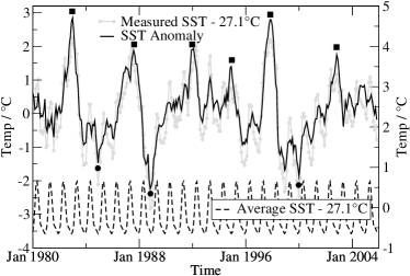
Figure 1: Observed ENSO SST oscillations since $1980$. The average (dashed black, right axis) and measured (grey, left axis) SST’s, minus $27.1^{\circ}$C, in the Niño $3.4$ region (cp. Fig. 2) with the SST anomaly (solid black, left axis). El Niño events are denoted by a black square above the event, La Niña events (see section II.3) by a black circle below.

Since 1899, there have been $29$ recorded El Niño events, giving an average period for ENSO of $3.7$ years KovBHW03 . However, there is evidence to suggest that El Niño events are becoming stronger and more frequent; there have been $6$ events in the last $20$ yrs (an average period of $3.3$ years), $2$ of which were the strongest of the century KovBHW03 ; NOAA .

II.1 Normal conditions

In order to understand the El Niño anomaly, let us first describe the normal conditions that exist in the Pacific Ocean between $120^{\circ}$ East and $90^{\circ}$ West. In Fig. 2 we show a schematic view of the relevant section of the Pacific.

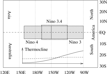
Figure 2: Schematic view of the Niño regions $3$ (right hashed rectangle), $4$ (left hashed rectangle) and $3.4$ (rectangle with dashed line borders). The thermocline height in normal (solid) and El Niño conditions (dashed line) is indicated schematically in the diagram.

In normal conditions, the trade winds blow from East to West across the tropical Pacific, resulting in warm surface water being pushed west, so that the thermocline — a region of water roughly $100$m below the surface where there is a very sharp temperature gradient separating the warm surface layer from the cold abyss — is depressed further in the West, and made shallower in the East Phi90 . The SST is about $8^{\circ}$C higher in the West, with cool temperatures off South America, due to cold water upwelling, i.e. rising from the deeper layer to the surface Mad00 . This cold nutrient-rich water supports diverse marine ecosystems and major fisheries, so upwelling is of immense ecological and economic importance to the west coast of the Americas NOAA ; COAPS .

The warmer SST in the West means increased evaporation and rising moist air, and hence high levels of rainfall (a tropical climate), along with low atmospheric sea-level pressures in the West. In the East, the colder SST results in far less rainfall, an arid inland climate and higher atmospheric sea-level pressures. This induced pressure difference drives the circulation of the trade winds. A measure of the strength of the trade winds is the Southern Oscillation Index (SOI), defined as the normalized difference in sea-level pressures between Tahiti and Darwin, Australia.

The whole process is a therefore a self-sustaining cycle; winds cause thermocline and SST changes, which cause pressure differences, which in turn drive the winds.

II.2 El Niño conditions

During an El Niño event the SST and SOI change dramatically. In the central and western Pacific, there is relaxation in the strength of the trade winds. This leads to a depression of the thermocline in the East and an elevation in the West, because less warm water is being pushed west. This increase in thermocline depth in the East can be as large as a factor of three, leading to an increase in SST, and the effective cut-off of upwelling of nutrients to the surface. This has devastating consequences for the primary producers (such as plankton) in the food chain, with knock-on effects for other life, such as fish and birdlife Phi90 .

The increased SST in the East also leads to an increased evaporation, and large amounts of rain, often causing extensive flooding. The rising air decreases the normally high pressure. During large El Niño events the SOI is very negative, indicating a reversal in trade winds. This causes a great deal of warm, moist air (and hence rain) to move east, whilst leaving a severe drought in the western Pacific, often resulting in large bush fires.

II.3 La Niña conditions

La Niña (The “Little Girl”) is the phase of the ENSO cycle which is opposite to El Niño. It is characterized by unusually cold ocean temperatures in the central and eastern Pacific. La Niña arises by a strengthening in the trade winds, further depressing the thermocline in the West (and elevating it in the East), which increases cold water upwelling in the eastern Pacific. This lower SST means the high levels of nutrients can support an abundance of life in the Ocean. The SOI is also positive (increased pressure difference), bringing enhanced rainfall in the West.

III The Delayed-Action Oscillator

III.1 A non-linear oscillator with delay term

The DAO is a simple non-linear model in which the ENSO effect is modeled by just three terms SuaS88 . With $T$ denoting the temperature anomaly, i.e. the deviation from a suitably defined long term average temperature, the model is given as a first-order, non-linear differential equation

$$\frac{dT}{dt}=\ kT-\ bT^{3}-\ {\cal A}T(t-\Delta)$$ (1)

with appropriate coupling constants $k$, $b$, ${\cal A}$ and $\Delta$. The first term on the right hand side in (1) represents a strong positive feedback within a coupled ocean-atmosphere system which is assumed to occur in the Niño $3.4$ region. A much deeper thermocline as in the West, or a cold SST as in the East, would result in much poorer feedback coupling. The feedback process works through advective processes giving rise to temperature perturbations which in turn result in atmospheric heating. This heating leads to surface winds, driving the ocean currents which will then enhance the anomaly $T$.

The second component is an unspecified nonlinear net damping term that is present in order to limit the growth of unstable perturbations. This term represents various ocean advective processes and moist processes that stop temperatures diverging.

Lastly, the model also considers equatorially-trapped ocean waves propagating across the Pacific, before interacting back with the central Pacific region after a certain time delay. These ocean waves are “hidden” Rossby waves which move westward on the thermocline, reflect off the rigid continental boundary in the West and then return eastward along the equator as Kelvin waves. Their respective wave velocities and the width of the Pacific basin determine the transit time, which is denoted $\Delta$ in Eq. (1). The strength of the returning, emerging signals relative to that of the local non-delayed feedback is denoted by ${\cal A}$. We also assume that $0<{\cal A}<k$ due to loss of information during transit and imperfect reflection.

We shall often use the DAO in its dimensionless form

$$\frac{dT^{\prime}}{dt^{\prime}}=\ T^{\prime}-\ (T^{\prime})^{3}-\ \alpha T^{\prime}(t^{\prime}-\delta),$$ (2)

where we have scaled time by $t^{\prime}=kt$ and temperature by $T^{\prime}=\sqrt{b/k}T$. The new constants then are $\alpha={\cal A}/k$ and $\delta=k\Delta$. In what follows, we shall for simplicity suppress the prime in all expressions where there is no ambiguity.

III.2 DAO wave propagation

The DAO delay term has a negative coefficient representing a negative feedback. To see the reason for this, let us consider a warm SST perturbation in the coupled region. This produces a westerly wind response that deepens the thermocline locally (immediate positive feedback), but at the same time, the wind perturbations produce divergent westward propagating Rossby waves that return after time $\Delta$ to create upwelling and cooling, reducing the original perturbation. This process can therefore be seen as a phase-reversing reflection off the coupled region; the resultant upwelling will cause further Rossby wave propagation, which in turn will cause downwelling and warming after a further delay, $\Delta$. Hence we expect the period of model oscillations to be no less that $2\Delta$ — “period doubling” SuaS88 .

Note that the eastern boundary will also contribute a delay term to the DAO, however equatorial Kelvin wave reflection from eastern boundaries is weak as the bulk of the wave propagates along the coast SoaWW99 . For this reason we may ignore these effects.

It is possible to estimate the wave transit times, and hence the time delay $\Delta$ of the DAO model, from knowledge of the wave speeds for Rossby and Kelvin waves (see Appendix A). We shall return to this direct comparison later, but for now we focus on the behavior of the dimensionless DAO (2).

III.3 Linear stability analysis

Equation (2) cannot be solved analytically. But we may study its dynamics by analyzing its behavior close the its fixed points, i.e. those special solutions $\bar{T}$ of (2) for which ${dT}/{dt}=0$ which also immediately implies $T(t)=T(t-\delta)$ for all $t$. Hence we need to solve

$$(1-\alpha)\bar{T}-\ {\bar{T}}^{3}=0$$ (3)

and so the fixed point solutions are $\bar{T}=0,\pm\sqrt{1-\alpha}$. $\bar{T}_{0}=0$ is the trivial fixed point, corresponding to a zero temperature anomaly. It is also unstable, i.e. any small perturbation will lead to a system moving away from $0$. Therefore we shall concentrate on the other two fixed points $\bar{T}_{\pm}=\pm\sqrt{1-\alpha}$. Due to symmetry, it is furthermore sufficient to consider one of these only and we choose $\bar{T}_{+}=\sqrt{1-\alpha}$.

The dynamics close to $\bar{T}_{+}$ can be examined by a linear stability analysis. Let us consider a small perturbation $S=T-\bar{T}_{+}$. Ignoring terms of more than linear order in $S$ SuaS88 , we find when substituting $S$ back into $(\ref{eq-DAOdimless})$ that

$$\frac{dS}{dt}=\ (3\alpha-2)S-\ \alpha S(t-\delta)$$ (4)

We now look for solutions of the form $S=Ae^{\sigma t}$, where $A$ is a constant real number equal the initial condition $S(0)$ and $\sigma$ is a complex number. Substituting this in (4) gives an equation for $\sigma$

$$\sigma=(3\alpha-2)-\ \alpha e^{-\sigma\delta}$$ (5)

Writing $\sigma=\sigma_{\rm R}+\imath\sigma_{\rm I}$, where $\sigma_{\rm R},\sigma_{\rm I}$ are both real, we find

$$\sigma_{\rm R} = (3\alpha-2)-\ \alpha\ \cos(\sigma_{\rm I}\delta)\ e^{-\sigma_{\rm R}\delta}$$ (6a)

$$\sigma_{\rm I} = \alpha\ \sin(\sigma_{\rm I}\delta)\ e^{-\sigma_{\rm R}\delta}$$ (6b)

When $\sigma_{\rm R}=0$, the solution $S=Ae^{\imath\sigma_{\rm I}t}$ is purely oscillatory and hence the fixed point is a center — neither stable nor unstable — with a finite frequency of $2\pi/\sigma_{\rm I}$. These neutral solutions occur along (an infinite number of) neutral curves of the form:

$$\delta=\frac{2n\pi\mp\arccos\left(\frac{3\alpha-2}{\alpha}\right)}{\sqrt{\alpha^{2}-\left(3\alpha-2\right)^{2}}}\ ,\qquad n\in\mathbb{N}\cup\{0\}$$ (7)

In Figure 3, we show the $(\alpha,\delta)$ phase diagram of the DAO obtained from the linear stability analysis.

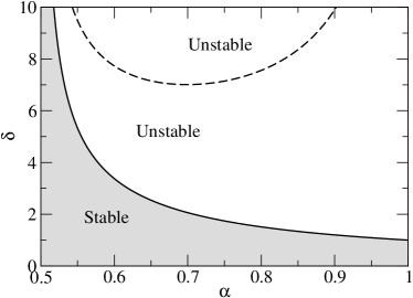
Figure 3: Phase diagram for the stability of fixed points $\bar{T}_{+}$. Neutral curves for $n=0$ (solid line) and $n=1$ (dashed line) are shown together with stable (grey) and unstable regions (white).

Only $0.5<\alpha<1$ is plotted, since for this domain the coefficient on the local term in $(\ref{eq-linearDAO})$ is always smaller than that of the delayed term. If it were larger, then the local term would always dominate, and the solution would always be stable, i.e. for $\alpha<0.5$ the fixed point is always stable and attracting, regardless of the initial conditions.

Choosing ($\alpha,\delta$) below the first neutral curve, e.g. within the shaded region of Figure 3, corresponds to $\sigma_{\rm R}<0$ and hence the solution is a decaying spiral — the fixed point is stable and attractive. However, taking ($\alpha$, $\delta$) above this neutral curve gives $\sigma_{\rm R}>0$, and so the perturbation spiral grows outwards — the fixed point is unstable and no matter how close to $T_{0}$ the solution starts, it will always move away.

If ($\alpha,\delta$) is taken above the second neutral curve, the fixed point is still unstable $(\sigma_{\rm R}>0)$ but the number of unstable modes has increased to two. However, the basic DAO equation (2) is only a one-dimensional problem, as there is only one variable $T$, and so the extra unstable modes do not influence the dynamics.

This linear stability approach is highly useful, given that it depends on only two parameters, $\alpha$ and $\delta$, and reveals valuable information about the stabilities of the fixed points. Given an $\alpha$ and a $\delta$, it also provides a solution to the DAO given by:

$$T(t)=\bar{T}_{+}+Ae^{\sigma_{\rm R}t}e^{\imath\sigma_{\rm I}t}$$ (8)

which is perfectly valid to within an order of ${\cal O}(T)$, provided it stays close to $\bar{T}_{+}$. However, once a solution is too far from an unstable fixed point or if the initial condition starts too far away from the fixed point, this linear stability approach breaks down. Figure 4 shows linear stability solutions for different $\delta$ values, given by Eq. (8), along with the full solutions discussed in Section III.4.

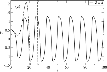
Figure 4: An $\alpha=0.75$ cross-section for $T$ vs $t$ for (a) a stable solution with $\delta=1$, (b) a nearly neutral solution at $\delta=2$ and (c) an unstable oscillation at $\delta=4$. Solid lines indicate numerical solutions for the anomaly $T$, dashed lines are obtained from the linear stability solutions $\bar{T}_{+}+S$. For clarity, we only plot the $\delta=4$ linear stability solution up to $t=30$.

III.4 Computation of full solutions by numerical integration

Let us now construct solutions to the DAO which are outside the region of validity of the linear stability analysis. As mentioned before, this is no longer possible analytically, so we will use numerical techniques to integrate up the time-behavior of (2). Fortunately, this involves the use of standard numerical tools available in a variety of mathematical software packages. For convenience, we have chosen the predefined Mathematica package NDelayDSolve Hay04 . The Mathematica code used to solve the basic DAO equation (2) is part of the code shown in Appendix B.

In Figure 4, we show the results obtained from Eq. (2) when carrying out this numerical procedure for $\alpha=0.75$ and various values of $\delta$. The initial value used is $T(0)=0.55$ which is close to the fixed point $\bar{T}_{+}=0.5$. In Fig. 5, we show the $(T,dT/dt)$ phase portraits for two values of $\delta$ close to the first neutral curve.

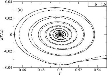
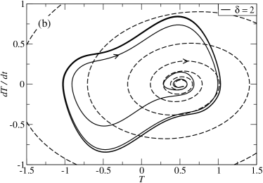
Figure 5: Phase portraits of $\frac{dT}{dt}$ vs $T$ with $\alpha=0.75$, solved up to $t_{\rm final}=100\delta$ with (a) $\delta=1.6$ and (b) $\delta=2$. Solid lines indicate numerical solutions of Eq. (2), dashed lines correspond to approximations obtained from the linear stability analysis. The arrows indicate the time flow.

Let us now briefly discuss the observed behavior. In Fig. 4(a), we see that the numerical solution and the linear approximation are in good agreement and quickly converge to the stable fixed point $\bar{T}_{+}=0.5$ as expected for $\delta=1$. In Fig. 4(b), we are still close to the neutral curve but have already crossed over into the unstable regime. Consequently, the numerical solution starts to slowly spiral away from $\bar{T}_{+}=0.5$, becoming large enough so that the dynamics are also influenced by the second unstable fixed point at $\bar{T}_{-}=-0.5$, resulting in the onset of oscillations between them. This is shown in more detail in Fig. 5(b). The agreement with the numerical solution clearly breaks down very quickly, since the linear stability analysis shows an unstable spiral, which continues to only grow about $\bar{T}_{+}$.

At an even larger $\delta$ value, we see in Fig. 4(c) that the numerical solution immediately diverges from the fixed point and goes to an oscillatory state, the amplitude of which is limited by the nonlinear damping term in Eq. (2).

The behavior for other values of $\alpha$ is analogous. Therefore, we have identified within the DAO model (2) a whole region of $\alpha$ and $\delta$ values where we obtain oscillations of the SST anomaly between a hot ($\bar{T}_{+}>0$) and a cold ($\bar{T}_{-}<0$) fixed point. This feature is what makes the DAO a model for oscillations between hot El Niño and cold La Niña conditions.

III.5 Comparing periodicities

As identified in the last section, the DAO model is capable of producing limit cycle oscillations for a wide region of ($\alpha,\delta$) values. We next compute the period of these oscillations and compare them to those observed for typical ENSO cycles.

As shown in Figure 2, the Niño $3.4$ region extends from $120^{\circ}$ West to $170^{\circ}$ West, with the midpoint at $145^{\circ}$ West. If we assume that the Pacific western boundary is at $\approx 120^{\circ}$ East, this gives an angular separation of $95^{\circ}$ of longitude for the waves to travel. This corresponds to a distance of $95(2\pi/360)r_{\rm Earth}=10.6\times 10^{6}$m, where the radius of the Earth $r_{\rm Earth}=6.37\times 10^{6}$m. Using the values of $1.4$ms^-1 for a Kelvin wave and $0.47$ms^-1 for the primary Rossby mode as obtained in Appendix A thus gives a delay of $262$ days for the Rossby propagation to the western boundary, and a further $87$ days for the return of the Kelvin waves, a total delay of $\Delta=349$ days.

This information now allows us to compute the time scaling parameter, however since $k=\delta/\Delta$, these are different for each value of $\delta$ used in the DAO model. By the use of a Fourier Transform applied over $600$ years, we find e.g. for $\alpha=0.7,\delta=3$ a period $\tau^{\prime}=11.1$ which corresponds to a true DAO period of $\tau=\tau^{\prime}/k=3.5$ years. In Fig. 6 we show the results of many runs with varying $\alpha=0.56,0.57,\ldots,1$ and $\delta=1,1.1,\ldots,4.9$.

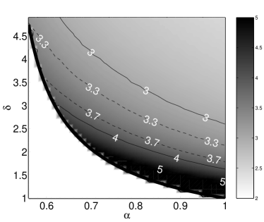
Figure 6: Grey scale plot of DAO periods for various $\alpha$ and $\delta$ values. Lines of constant periods are indicated, those corresponding to periods $3.3$ and $3.7$ are shown as dashed lines. The white region corresponds to the stable region as present in Fig. 3, with the thick black line representing the first neutral curve.

Comparing these periods to real ENSO events, which have a period of $3.3$ to $3.7$ years, we see that there is a large region of $(\alpha,\delta)$ values where there is a good agreement.

III.6 Discussion of the basic DAO model

In the preceding sections, we have seen that the DAO is a useful tool in studying the ENSO cycle. The main beauty of the DAO (1) is its simplicity. Although the full equation cannot be solved explicitly, the linear stability analysis and the numerical solutions both give highly useful insights. In particular, the numerical solutions exhibit the true global dynamics of the DAO. There are limit cycle oscillations, with a period that matches the real world, and hence the DAO is a good model for these features of ENSO. Nevertheless, the DAO model assumes a localized coupled problem, which is obviously an over-simplification of the situation in the Pacific. All influences of the atmosphere, the earth’s rotation, and the ocean currents and dynamics are simply modeled by a non-linear, effective damping term and a somewhat arbitrary delay. The delay term ignores, e.g. East boundary reflections that could possibly be considered. The model further assumes that time scales must be related to propagation times of equatorially trapped oceanic waves in a closed basin. For the atmosphere, which has short time scales, the DAO simply assumes an instantaneous response.

IV Annual Forcing

In this and the following sections, we shall extend the basic DAO discussed above by including external influences which allow us to model the ENSO dynamics better. In order to distinguish this extended DAO from its original, we shall denote the new model as ENSO-DAO from now on.

IV.1 Modifying the DAO to include the annual cycle

As mentioned above, an El Niño event typically appears in late December, early January. Thus the annual cycle is clearly playing an important role in determining the onset of El Niño ZebC87 ; Str99 . Let us thus add to the DAO (1) another term that models the periodic heating and cooling of the equator during the annual cycle. The average SST data, as shown on Fig. 1, can be used to construct a Mathematica interpolating function, $Y(t)$, representing the continuous changes of the average SST during the year . We therefore include its numerical time derivative, representing the expected change in SST due to annual forcing, to give a new DAO equation

$$\frac{dT}{dt}=\ kT-\ bT^{3}-\ {\cal A}T(t-\Delta)+\frac{d}{dt}Y(t)$$ (9)

This equation now depends critically on the $(\alpha,\delta)$ values chosen in the dimensionless model, since computation of the scaling constants $k$ and $b$ is required. We have seen earlier that $k=\delta/\Delta$, and $b$ is given by the expression $b=k(T^{\prime}/T)^{2}$. In order to estimate $b$ we shall take $T^{\prime}/T$ as the ratio of their respective maxima/minima. Figure 1 shows the maximum anomaly is on average $2^{\circ}$C, whilst the maximum value of $T^{\prime}$ can be calculated for any values $(\alpha,\delta)$.

Choosing $\alpha=0.7,\delta=3$ as the standard ENSO-DAO model for the next few sections allows us to calculate $k=3.14$/years, $b=1.09$ ^∘C^-2/years, and hence discuss the behavior of this specific model under annual forcing.

IV.2 Solving the annually forced DAO

Fixed points of (9) do not exist; they are now fixed cycles fluctuating about $0,\pm\sqrt{(k-{\cal A})/b}$ due to the periodic nature of the forcing term. Nevertheless, taking $t=0$ to be the start of the year, the expected SST will be at its coldest and $dY/dt=0$, so we can take the initial condition to be $T(0)=\sqrt{(k-{\cal A})/b}+0.15$ (this is similar to before but now includes the scaling constants).

Let us now consider numerical solutions of Eq. (9). In Fig. 7, we show the solution of $T$ vs $t$ for parameters as above. The annual cycle as in Fig. 1 is also shown.

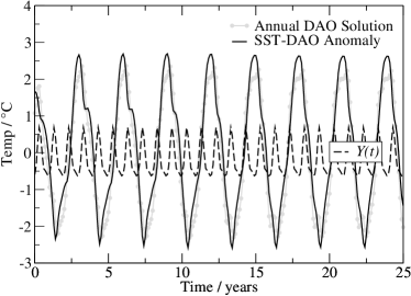
Figure 7: Numerical solution of the annually forced DAO (9) with $\delta=3$ and $\alpha=0.7$ showing the annual cycle $Y(t)$ (dashed black), model solution $T$ (grey) and SST anomaly $T-Y(t)$ (solid black).

We note that with the inclusion of annual forcing, $T$ is no longer the SST anomaly, but rather, the anomaly is the difference between $T$ and the annual forcing, $Y(t)$. This true SST anomaly is also shown in Fig. 7, and should be compared to Fig. 1.

From Fig. 7 it is clear that the addition of an annual forcing term has changed the dynamics in several ways. Firstly, the peak amplitude of the oscillations has been increased. The peaks themselves are less regular because of the quickly changing forcing term provided by the seasons. However, the paramount effect of the annual cycle is in determining the onset and period of an El Niño event. Hot events only occur in-phase with the annual cycle, and hence the ENSO-DAO now has an exact integer period, e.g. 3 years for our model. The ENSO-DAO gives high temperatures from July through to March of the next year — which is indeed as observed in the Pacific — with the maximum amplitude usually in December.

V Global Warming

Global warming is another effect that may influence the periodicity and amplitude of ENSO events. For the purpose of this paper it will be modeled via a constant heating on the Pacific DAO system. Working with the dimensionless DAO for simplicity, this is achieved by adding a constant $\beta$ to the DAO equation (2) giving:

$$\frac{dT}{dt}=\ T-\ T^{3}-\ \alpha T(t-\delta)+\ \beta$$ (10)

On its own, this term would give $\frac{dT}{dt}=\beta$, solved by $T=\beta t+c$, a linear warming with time. We shall consider $\beta>0$, a constant heating, although $\beta<0$ cooling can be treated completely analogously.

Current climate change models predict the rise in average global temperature over the next $100$ years will be below $5^{\circ}$C JohGIJ03 , hence we chose this scenario to be used in our ENSO-DAO. Using the standard model of Section IV, this gives

$$\beta_{\rm global\ warming}=k^{-1}\sqrt{\frac{b}{k}}\ \frac{5^{\circ}\mbox{C}}{100\mbox{years}}=0.009$$ (11)

as the value of $\beta$ in Eq. (10).

V.1 Fixed points, linear stability analysis and consequences

The fixed point solutions are now determined by the equation:

$$(1-\alpha)\bar{T}^{(\beta)}-\left(\bar{T}^{(\beta)}\right)^{3}+\beta=0$$ (12)

For small $\beta$, there is hardly any change from the original $\bar{T}$ fixed points, and hence the system will behave as the basic DAO. As $\beta$ is increased, the unstable inner fixed point $\bar{T}^{(\beta)}_{0}$ decreases from zero, whereas both the outer solutions $\bar{T}^{(\beta)}_{\pm}$ increase. In cases when $\beta$ is large, and for large enough $\alpha$, only one fixed point remains on the real axis (the other two are now complex).

Instead of considering solutions starting near $\bar{T}_{+}=\sqrt{1-\alpha}$, we now start near $\bar{T}^{(\beta)}_{+}$. The neutral curves can be determined via the same methods used to obtain Eq. (7), but with the fixed point $\bar{T}^{(\beta)}_{+}$ now depending on $\beta$:

$$\delta=\frac{2n\pi\mp\arccos\left[\frac{1-3\left(\bar{T}^{(\beta)}_{+}\right)^{2}}{\alpha}\right]}{\sqrt{\alpha^{2}-\left[1-3\left(\bar{T}^{(\beta)}_{+}\right)^{2}\right]^{2}}}\ ,\qquad n\in\mathbb{N}\cup\{0\}$$ (13)

The first neutral curve for a $\beta_{\mathrm{global\ warming}}$ DAO system, compared to no heating, is plotted in Fig. 8.

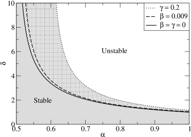
Figure 8: The first neutral curve for the original DAO (solid black, as in Fig. 3), forced DAO (dashed black) and symmetrically coupled DAO (dotted black). Also shown is the stability region affected by global warming (hashed), and by coupling (dotted). Higher mode neutral curves are not shown.

Consider a basic DAO system (above the solid black neutral curve in Figure 3) that has an unstable fixed point $\bar{T}^{(\beta=0)}_{+}$ with limit cycle oscillations. By introducing $\beta>0$, the neutral curve is shifted to the right, and hence the additional (hashed) stable region in Fig. 8 is created, changing the DAO dynamics. As $\beta$ increases, the model fluctuates for longer about the unstable $\bar{T}^{(\beta)}_{+}$ before flipping out to oscillate around both fixed points. Eventually, the dashed neutral curve in Fig. 8 moves to the right of ($\alpha,\delta$) and $\bar{T}^{(\beta)}_{+}$ becomes attracting. This stability bifurcation occurs at $\beta_{\mathrm{bif}}$, which can be found for any given ($\alpha,\delta$) by solving Eq. (13) for $\beta$.

If enough heating were applied to the DAO, the ENSO cycle would be terminated, leaving an ocean at a constant temperature and with no El Niño events. However, for slow heating, such as $\beta=0.009$, there is very little change to the time dependence of the DAO with respect to SST anomaly amplitudes or their periodicity except for a small subset of solutions. This would suggest that global warming will not affect ENSO, and hence El Niño events will still continue to occur.

VI Stochastic Effects

Chaos inherent in real world weather systems plays an important part in the irregularity of El Niño events. Processes such as storms, cyclones and ocean currents which traverse the Pacific play no part in our ENSO model, but will influence the system for their duration in the Niño $3.4$ region. We therefore consider the addition of a general stochastic term Has76 $R(t)$ to the dimensional DAO equation (1) giving:

$$\frac{dT}{dt}=\ kT-\ bT^{3}-\ {\cal A}T(t-\Delta)+\ R(t)$$ (14)

$R(t)$ is a step function that takes fixed, normally distributed (mean $0$, standard deviation $\lambda$), random values for each monthly time-step. A (non-ENSO) event that lasts for longer than one month is unphysical, and shorter-lived events will not have time to cause any significant differences (their randomness is averaged out).

Another way of viewing $R(t)$ is as a $\beta$ heating/cooling that only lasts for one month. This will mean that the neutral curves given by Eq. (13) will shift right/left each month, due to the fixed points $\bar{T}^{(R)}_{\pm}$ changing position.

If $\lambda$ is small, then there is hardly any change to the basic DAO. However, for large enough $\lambda$, the fixed points can change their stabilities each month, inducing a great deal of random behavior in the DAO. For example, the system may be stable and tending towards $\bar{T}^{(R)}_{+}$ of that month, and then $R(t)$ changes to produce an unstable system that wants to oscillate. This creates many different El Niño events with differing amplitudes and durations, as well as the possibility of times where the system stays near zero.

VII The full ENSO-DAO

We now combine of all of the effects considered above, namely the annual cycle, global warming and stochastic effects. Therefore the DAO equation (1) becomes

$$\frac{dT}{dt}=\ kT-\ bT^{3}-\ {\cal A}T(t-\Delta)+\ Y^{\prime}(t)+\ {\cal B}+\ R(t)$$ (15)

Using the standard model of Section IV, with ${\cal B}=5^{\circ}\mbox{C}/100$years as the fully dimensional global warming factor and $R(t)$ with $\lambda=5$, the DAO produces very realistic pictures, such as Fig. 9, that look remarkably similar to Fig. 1.

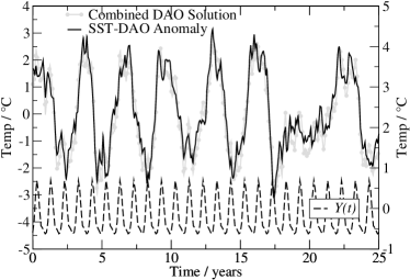
Figure 9: Numerical solution of the combined DAO (15) with $\delta=3$ and $\alpha=0.7$ showing the annual cycle $Y(t)$ (dashed black, right axis), model solution $T$ (grey, left axis) and SST anomaly $T-Y(t)$ (solid black, left axis).

Most obvious are the small fluctuations associated with the stochastic effects. In addition, the regularity of the original DAO oscillations is broken and sometimes a complete ENSO event has vanished. E.g. the absence of the SST peaks at about $t\sim 20$ in Fig. 9. This happens when the onset of the ENSO cycle event takes place at a time when the random forcing happens to change the SST into the opposite direction. We emphasize that a variety of solution curves similar to Fig. 9 can be generated by taking other ($\alpha,\delta$) combinations, initial SST values and stochastic forcing.

VIII Coupled DAOs

The basic DAO model (1) considers a single, but representative region with strong atmospheric-ocean coupling in the Pacific. Clearly, we might also want to consider situations in which other regions of the Pacific are incorporated. These could be either other regions along the equator, where we would expect differing coupling strengths and delay times. Or they could be regions to the North and South of the central DAO region in which no delay and only weak coupling exists, such that these additional regions act as temperature sinks. Possible arrangements are shown in Fig. 10. In this chapter, we will consider one such prototype situation, namely two coupled regions along the equator.

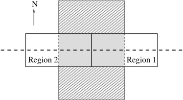
Figure 10: Schematic of the Pacific showing the original ENSO-DAO region (grey), new coupled regions $1$ and $2$ and potential North–South regions (hashed). The equator is indicated as a horizontal dashed line.

VIII.1 Two coupled DAOs along the equator

Let us for simplicity assume that coupling $\alpha$ and delay $\delta$ in the two regions are the same. This is a valid assumption as long as the two adjacent regions are both in the strong-coupling region such that the distance to the Western boundary is approximately the same, with the same losses and reflection properties. If one region is warmer than the other, then the flow of heat energy across their common boundary will act to heat one and cool the other. This can be modeled by incorporating a $\gamma T_{i+1}$ term in each DAO with $\gamma>0$ and $T_{i+1}$ the anomaly in the adjacent DAO region. Then we have a system of $2$ coupled DAOs such that

$$\frac{dT_{1}}{dt}=\ T_{1}-\ {T_{1}}^{3}-\ \alpha T_{1}(t-\delta)+\gamma T_{2}$$ (16a)

$$\frac{dT_{2}}{dt}=\ T_{2}-\ {T_{2}}^{3}-\ \alpha T_{2}(t-\delta)+\gamma T_{1}$$ (16b)

The fixed point solutions can be found as before by taking $\frac{dT_{i}}{dt}=0$ and substituting (16a) into (16b). This yields a $9$th order polynomial in $\bar{T}^{(\gamma)}_{i}$ with a mixture of real and complex roots which vary as a function of $\gamma$. The solutions $\bar{T}^{(\gamma)}_{i\pm}=\pm\sqrt{1-\alpha+\gamma}$ are the same in both regions and are always real since $0<\alpha<1$, and hence are of most interest.

Conducting a linear stability analysis about the fixed points ($\bar{T}^{(\gamma)}_{1+}$, $\bar{T}^{(\gamma)}_{2+}$) as in Section III.3, we find neutral curves given by

$$\delta=\frac{2n\pi\mp\arccos\left(\frac{3\alpha-2-2\gamma}{\alpha}\right)}{\sqrt{\alpha^{2}-\left(3\alpha-2-2\gamma\right)^{2}}}\ ,\qquad n\in\mathbb{N}\cup\{0\}$$ (17)

The first neutral curve is shown in Figure 8 for an example with $\gamma=0.2$.

We see that similar to Section V, the neutral curves move right with increasing $\gamma$, such that the fixed point can bifurcate from unstable to stable. So, if there is strong coupling between regions in the Pacific (large $\gamma$), then independent oscillations cannot occur and the system settles down to constant temperature anomalies. However, for sufficiently weak coupling, ENSO-style oscillations are still permitted.

As before, we have also solved the Eq. (16) numerically. Depending on the initial SST anomalies, we find that we can drive the regions into (i) stable, non-oscillatory solutions, (ii) in-phase oscillations and even (iii) oscillations which are out-of-phase by $\pi$. For brevity, we do not show the results here.

VIII.2 Two regions with different ENSO coupling

Let us now consider briefly the situation in which $\alpha_{i}$ or $\delta_{i}$ are different in the different regions. If $T_{2}$ represents the anomaly in region $2$ of Fig. 10 and $T_{1}$ the anomaly in region $1$, then the wave transit time from $T_{1}$ to the western boundary would be greater than that from $T_{2}$. Similarly, the strength of the returning signal to $T_{1}$ would be less than that to $T_{2}$, as more information would be lost due to the greater distance across which information is transported. However, the waves propagating from $T_{1}$ are not hidden from the problem whilst they are propagating through $T_{2}$, suggesting that $\delta$ could be the same for both regions, namely the propagation time from $T_{2}$ to the western boundary and back. Similarly, the strength of the local coupling is assumed to be less in $T_{1}$, suggesting that even though the strength of the returning signal is less, relative to the local coupling its affect would be the same as in $T_{2}$. Figure 11 shows how the coupled model (16) is affected by different values of $\alpha$.

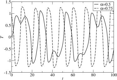
Figure 11: Numerical solutions to the coupled DAO (16), with $\alpha_{1}=0.5$ in region $1$, $\alpha_{2}=0.75$ in region $2$, $\delta=4$ in both regions and $\gamma=0.1$.

In the Figure we see that $T_{1}$ shows some irregular behavior with varying amplitudes. This behavior is more like that of El Niño than the simple DAO.

Other possible coupled DAO scenarios could include $3$ coupled regions, either along the equator or aligned along a south-north axis. Our preliminary results indicate that such models gives rise to irregular ENSO cycles as above. However, the models have to be treated with proper care, since some solutions become unphysical, e.g. indicating uninterrupted heating or cooling of the ocean.

IX Conclusions

The DAO is given by a simple one-dimensional differential equation, and may nowadays be studied by readily available desk- or laptop computing facilities. Yet it captures much of the observed richness and variance of the ENSO phenomenon. We are therefore convinced that it presents an ideal tool to introduce students to the topic. Let us briefly recapitulate what issues we have been able to study in the present paper using the DAO. We first outline the linear stability analysis and the numerical solution of the DAO that were the content of the first paper on the DAO SuaS88 . This then serves to introduce the concept of shallow-water Kelvin and Rossby waves, as well as to establish our notation. Using the corresponding wave speeds and the geography of the Pacific, we can already show that for a large set of parameters, the observed ENSO periodicity can be modeled by the DAO.

Next, the inclusion of the measured annual cycle demonstrates that the observed ENSO-DAO periodicity may in fact be heavily influenced by the Earth’s period around the Sun. The occurrence of an ENSO event is very much subject to the right season and thus the original DAO period need not be identical to the observed ENSO-DAO period. We stress that the modeling of the annual cycle within the DAO is quite easy and should not be beyond any student who has mastered the original DAO.

We then extended the DAO to include a constant heating — global warming — and found that current predictions of $5^{\circ}$C rise over $100$ years are unlikely to influence the ENSO-DAO dynamics. We also do not find any large increase in either occurrence or magnitude of ENSO events. This seems to be at variance with current predictions based on CGCMs VogL98 ; TimOBE99 and might just indicate the limitations of the ENSO-DAO model for true, quantitative predictions .

Putting it all together, we then included a certain level of stochastic forcing alongside the annual cycle, and found that the ENSO-DAO dynamics now become very much like the observed ENSO dynamics, showing a large variation in oscillation periods and amplitudes. At least on a qualitative level — the range of the SST oscillations is in fact even quantitatively similar — which shows the strength of the ENSO-DAO.

Finally, we briefly discussed some extensions of the ENSO-DAO model, such as coupled regions. The example of the $2$-coupled-regions model shows that the extended DAOs share some irregularities with the observed ENSO phenomenon already, even in the absence of annual or stochastic forcing. Further investigations of ENSO-DAO might include an analysis of the statistical properties of the measured ENSO cycles as in Fig. 9 and comparisons with observed data, a more thorough analysis of the possible changes in periodicity and strengths of ENSO-DAO oscillations due to human influences, a mathematical analysis of the DAO for integer periods or even an application to the Atlantic.

In conclusion, we see that the DAO — while being a research tool in its own right WhiTBD03 — can be investigated by modest analytical and computational resources. We think that it will be an ideal topic for all students, teachers and lecturers interested in the exciting dynamics of the El Niño phenomenon and hope that the present paper will help them in this quest.

Appendix A Shallow water equations and waves

A.1 Two-fluid model and shallow water equations

Oceans are warmer near the surface than they are in the deep, and due to thermal expansion this warm layer will have a lower density. Thus a simple model for the ocean structure is a two-fluid model with density $\rho_{1}$ in the warm surface layer and density $\rho_{2}>\rho_{1}$ below in the cold abyss. The dividing zone is called the thermocline. At its widest, the Pacific is $17,700$km across from the Malay Peninsula to Panama whilst only having an average depth of $4,280$m. So the Pacific is roughly $3$ orders of magnitude wider than it is deep, and so we are justified in rewriting the original Navier-Stokes equations using the shallow-water approximation Gil82 ; Hol04 . These are given as

$$\frac{\partial\eta}{\partial t}+H\left(\frac{\partial u}{\partial x}+\frac{\partial v}{\partial y}\right) = 0$$ (18a)

$$\frac{\partial u}{\partial t}+u\frac{\partial u}{\partial x}+v\frac{\partial u}{\partial y}-fv+g^{\prime}\frac{\partial\eta}{\partial x} = 0$$ (18b)

$$\frac{\partial v}{\partial t}+u\frac{\partial v}{\partial x}+v\frac{\partial v}{\partial y}+fu+g^{\prime}\frac{\partial\eta}{\partial y} = 0$$ (18c)

in the absence of external forces. Here $(u,v,w)$ is the displacement velocity in the Cartesian frame $(x,y,z)$ and $\eta(x,y,t)$ is a small perturbation to the constant mean thermocline depth $H$. Furthermore, $f$ is the Coriolis parameter and $g^{\prime}=\frac{\rho_{2}-\rho_{1}}{\rho_{1}}g$ is the effective gravitational acceleration. Equations (18) permit two types of thermocline wave solutions. The first are inertia-gravity Kelvin waves. The second type are planetary Rossby waves.

A.2 Kelvin waves

Equatorially trapped Kelvin waves have no meridional ($y$) velocity fluctuations such that the shallow water equations (18) can be simplified to

$$\frac{\partial^{2}u}{\partial t^{2}}-g^{\prime}H\frac{\partial^{2}u}{\partial x^{2}}=0$$ (19a)

$$f\frac{\partial u}{\partial t}-g^{\prime}H\frac{\partial^{2}u}{\partial x\partial y}=0$$ (19b)

Equation (19a) implies that solutions have to be of the form $u=E(y)F(x\pm ct)$ with wave speed $c=\sqrt{g^{\prime}H}$. In addition, Eq. (19b) prohibits westward propagation ($F(x+ct)$) since those solutions become unbounded at large $y$. Therefore only eastward, equatorially trapped ($v=0$), Kelvin waves are possible. These non-dispersive thermocline gravity waves propagate eastward with speed $c\approx 1.4$ms^-1, when assuming a height $H=100$m and $(\rho_{2}-\rho_{1})/\rho_{1}=0.002$ Phi90 for the two-fluid model .

A.3 Rossby waves

Rossby waves owe their existence to the variation of the Coriolis parameter with latitude. Close to the equator the Coriolis parameter is given by $f=2\Omega y/r_{\rm Earth}$ where $r_{\rm Earth}$ is the radius of the Earth and $\Omega$ the Earth’s angular velocity. If we consider a linearized version of the shallow-water equations and seek solutions for latitudinal waves of the form $v=V(y)\exp{\imath(kx-\omega t)}$, with $\omega>0$ and the sign of $k$ determining the direction of zonal ($x$) phase propagation, we obtain their wave equation as

$$\frac{\partial^{2}V}{\partial y^{2}}+\frac{\beta^{2}}{g^{\prime}H}\left(Y^{2}-y^{2}\right)V=0$$ (20)

with

$$Y^{2}=\frac{g^{\prime}H}{\beta^{2}}\left(\frac{\omega^{2}}{g^{\prime}H}-k^{2}-\frac{\beta k}{\omega}\right)$$ (21)

and $\beta=2\Omega/r_{\rm Earth}$. From (20) we see that solutions are wavelike within an equatorial waveguide of width $2Y$, and decay exponentially for latitudes greater than $|Y|$.

If we now assume that the latitudinal dependance of $V$ is of plane-wave type $\sim\exp(\imath ny)$, then for these equatorially trapped waves we have $n\in\mathbb{N}$ as the only allowed standing wave solutions. A dispersion relation can be extracted from (20) and at low frequencies

$$\omega=\frac{-\beta k}{k^{2}+\frac{2n+1}{\lambda^{2}}}\ \ ,\ \quad n\in\mathbb{N}$$ (22)

with wavelength $\lambda=\sqrt{c/\beta}$. Since $k$ must therefore be negative, all Rossby waves have westward phase propagation. The slow, short, dispersive waves have eastward group velocities and the fast, long, non-dispersive waves have westward group velocities of $c/(2n+1)$. Only the long waves are important in the oceanic adjustment to changes in surface winds — a process that is crucial in ocean-atmosphere coupled systems — so only westward propagating Rossby waves will usually be considered.

The fastest Rossby wave ($n=1$) travels at one third the speed of a Kelvin wave, e.g. $\approx 0.47$ms^-1 in the Pacific. These are the non-dispersive, equatorially trapped, westward propagating Rossby waves considered in the DAO model in Section III.

Appendix B Numerical Routines

We include an abbreviated, but fully functional Mathematica 5.2 code for the solution of the annually forced DAO with global warming and monthly random weather as studied in Section VII. Physical units used in the code are given in years for time and Kelvin for temperature throughout.

<<NDelayDSolve.m

(* Define the variables to be used and calculate
   the required scalings *)

year=365.24; delay=349/year; alpha=0.7; delta=3;
beta=0.05; k=delta/delay; time=25;

(* Solve the basic dimensionless DAO, determine its
   maxima and therefore the value of b, the
   temperature scaling *)

Tfp=Sqrt[1-alpha];
orig= NDelayDSolve[
       {T’[t] == T[t]-T[t]^3-alpha*T[t-delta]},
       {T->(Tfp+0.05&)},
       {t,0,25*delta},
       MaxRecursion->50
      ];
values=Table[T[t]/.orig,{t,0,25*delta,0.1}];
Tmax=Max[values];
b=k*(Tmax/2)^2;

(* Read the real data from file, and construct
   annual cycle function *)

data=ReadList["ave_sea_temp.txt"];
yearly = Interpolation[data-27.1,
          PeriodicInterpolation->True];
Y[t_]:=yearly[ 12*t +1 ]

(* Create a Gaussian Distributed random variable
   (mean zero, standard deviation lambda) which
   changes every month, representing the effects
   of stochastic processes on the DAO *)

lambda=5;
Needs["Statistics’ContinuousDistributions’"];
stochastic=Table[Random[
       NormalDistribution[0,lambda]],{time*12+1}
       ];

R[t_]:= stochastic[[IntegerPart[12*t]+1]];
Plot[R[t],{t,0,time}]

(* Solve the Combined DAO Equation *)

Tf = Extract[T /.
  Solve[k*T - b*T^3 - k*alpha*T + beta == 0, T],
 3];

combo =
 NDelayDSolve[
  {(T’)[t] == k*T[t] - b*T[t]^3
   - k*alpha*T[t - delta/k]
   + beta + R[t] + (Y’)[t]},
   {T->((Tf + 0.15 &))
  },
  {t, 0, time},
  MaxRecursion -> 100, MaxSteps -> Infinity
 ];

(* Plot the Combined DAO Solution, the Annual Cycle,
   and the SST-DAO Anomaly *)

Plot[
 {Evaluate[T[t]/.combo],Y[t],Evaluate[T[t]/.combo]
   -Y[t]},{t,0,time},
  AxesLabel->{"t/years","T/K"},
  PlotStyle->{{RGBColor[0,1,0]},
              {RGBColor[0,0,0]},
              {RGBColor[1,0,0]}}
];

(* Calculate the period of the anomaly
   oscillations using Fourier Transform method *)

data=Abs[Fourier[Table[(T[t]/.combo)-Y[t],
    {t,0,time,0.1}]]];
Do[If[data[[k]]==Max[data],ans=Return[k]],
    {k,1,time,1}];
period=N[time/(ans-1)]

References

- (1) Oswald Blackwood, American Journal of Physics 11, 349 (1943).
- (2) B. Schmittmann and R. K. P. Zia, American Journal of Physics 67, 1269 (1999).
- (3) CNN, El Niño returns: an online companion to CNN’s special coverage, http://www.cnn.com/SPECIALS/el.nino/, 1997.
- (4) Curt Suplee, National Geographic Magazine (1998), http://www.nationalgeographic.com/elnino/mainpage.html.
- (5) Mark Saunders, El Niño and La Niña: Impacts and Predictions, BBC Weather, 2001, http://www0.bbc.co.uk/weather/features/el_nino2.shtml.
- (6) J. Picaut, F. Masia, and Y. du Penhoat, Science 277, 663 (1997).
- (7) K.-M. Kim and K.-M. Lau, http://atmospheres .gsfc.nasa.gov/contact/work/tbo/tbogrl.pdf (2000).
- (8) Max J. Suarez and Paul S. Schopf, J. Atmos. Sci. 45, 3283 (1988).
- (9) Warren B. White, Yves M. Tourre, Mathew Barlow, and Mike Dettinger, Journal of Geophysical Research 108, 3070 (2003).
- (10) G. Burgers and D.B. Stephenson, Geophys. Res. Lettrs, 26, 1027 (1998).
- (11) S. George Philander, El Niño, La Niña, and the Southern Oscillation, Vol. 46 of International Geophysics Series (Academic Press, London, 1990).
- (12) National Oceanic and Atmospheric Administration, NOAA El Niño Home Page, http://www.elnino.noaa.gov/.
- (13) Center for Ocean-Atmospheric Prediction Studies, El Niño and La Niño Home Page, http://www.coaps.fsu.edu/lib/elninolinks/.
- (14) R. Sari Kovats, Menno J. Bouma, Shakoor Hajat, Eve Worrall, and Andy Haines, The Lancet (2003).
- (15) Pierre Madl, Environmental Physics 437 (2000).
- (16) J. Soares, I. Wainer, and N. C. Wells, Ann. Geophys. 17, 827 (1999).
- (17) Allan Hayes, NDelayDSolve.m, Wolfram Research, 2004, http://library.wolfram.com/infocenter/MathSource/725/.
- (18) Stephen E. Zebiak and Mark A. Cane, Mon. Wea. Rev. 115, 2262 (1987).
- (19) David Strozzi, BA thesis, Princeton University, 1999.
- (20) T.C. Johns, J.M. Gregory, W.J. Ingram, C.E. Johnson, A. Jones, J.A. Lowe, J.F.B. Mitchell, D.L. Roberts, D.M.H. Sexton, D.S. Stevenson, S.F.B. Tett, and M.J. Woodage, Climate Dynamics 20, 583 (2003).
- (21) K. Hasselmann, Tellus 28, 473 (1976).
- (22) Gretchen Vogel and Andrew Lawler, Science 280, 1684 (1998).
- (23) A. Timmermann, J. Oberhuber, A. Bacher, M. Esch, M. Latif, and E. Roeckner, Nature 398, 694 (1999).
- (24) Adrian E. Gill, in Atmosphere-Ocean Dynamics, Vol. 30 of International Geophysics Series, edited by William L. Donn (Academic Press, San Diego, 1982).
- (25) James R. Holton, An Introduction to Dynamic Meteorology, Vol. 88 of International Geophysics Series (Elsevier Academic Press, San Diego, 2004).
- (26) S. Fred Singer, Is There a Connection Between El Niño and Global Temperatures?, http://www.sepp.org/scirsrch/elnino.html, (1999).