Power-law Strength-Degree Correlation From a Resource-Allocation Dynamics on Weighted Networks

Abstract

Many weighted scale-free networks are known to have a power-law correlation between strength and degree of nodes, which, however, has not been well explained. We investigate the dynamic behavior of resource/traffic flow on scale-free networks. The dynamical system will evolve into a kinetic equilibrium state, where the strength, defined by the amount of resource or traffic load, is correlated with the degree in a power-law form with tunable exponent. The analytical results agree well with simulations.

I Introduction

A very interesting empirical phenomenon in the study of weighted networks is the power-law correlation between strength $s$ and degree $k$ of nodes $s\sim k^{\theta}$ Li2004 ; Barrat2004a ; Wang2005a ; Liu2006 . Very recently, Wang et al have proposed a mutual selection model to explain the origin of this power-law correlation Wang2005b . This model can provide a partial explanation for social weighted networks, that is, although the general people want to make friend with powerful men, these powerful persons may not wish to be friendly to them. However, this model can not explain the origin of power-law strength-degree correlation in weighted technological networks.

In many cases, the concepts of edge-weight and node-strength are associated with network dynamics. For example, the weight in communication networks is often defined by the load along with the edge Newman2004 , and the strength in epidemic contact networks is defined by the individual infectivity Zhou2006 . On the one hand, although the weight/strength distribution may evolve into a stable form, the individual value is being changed with time by the dynamical process upon network. On the other hand, the weight/strength distribution will greatly affect the corresponding dynamic behaviors, such as the epidemic spreading and synchronization Yan2005 ; Motter2005 ; Chavez2005 ; Zhao2006 .

Inspired by the interplay of weight and network dynamics, Barrat, Barthélemy, and Vespignani proposed an evolution model (BBV model for short) for weighted networks Barrat2004b ; Barrat2004c . Although this model can naturally reproduce the power-law distribution of degree, edge-weight, and node-strength, it fails to obtain the power-law correlation between strength and degree. In BBV model, the dynamics of weight and network structure are assumed in the same time scale, that is, in each time step, the weight distribution and network topology change simultaneously. Here we argue that the above two time scales are far different. Actually, in many real-life situations, the individual weight varies momently whereas the network topology only slightly changes during a relatively long period. Similar to the traffic dynamics based on the local routing protocol Holme2003 ; Tadic2004 ; Yin2006 ; Wang2006 , we investigate the dynamic behaviors of resource/traffic flow on scale-free networks with given structures, which may give some illuminations about the origin of power-law correlation between strength and degree in weighted scale-free networks.

II Resource flow with preferential allocation

As mentioned above, strength usually represents resources or substances allocated to each node, such as wealth of individuals of financial contact networks Xie2005 , the number of passengers in airports of world-wide airport networks Guimera2005 , the throughput of power stations of electric power grids Albert2004 , and so on. These resources also flow constantly in networks: Money shifts from one person to another by currency, electric power is transmitted to every city from power plants by several power hubs, and passengers travel from one airport to another. Further more, resources prefers to flow to larger-degree nodes. In transport networks, large nodes imply hubs or centers in traffic system. So passengers can get a quick arrival to the destinations by choosing larger airports or stations. In financial systems, people also like to buy stocks of larger companies or deposit more capital in the banks with more capital because larger companies and banks generally have more power to make profits and more capacity to avoid losses. Inspired by the above facts, we propose a simple mechanism to describe the resource flow with preferential allocation in networks.

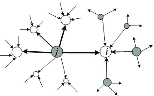
Figure 1: Resources in node $j$ are divided into several pieces and then flow to its neighbors. The thicker lines imply there are more resources flowing. It is worth pointing out that, in order to give a clearer illustration we do not plot the resource flow into node $j$ or out of node $i$.

At each time, as shown in Fig. 1, resources in each node are divided into several pieces and then flow to its neighbors. The amount of each piece is determined by its neighbors’ degrees. We can regulate the extent of preference by a tunable parameter $\alpha$. The equations of resource flow are

$$Q_{j\rightarrow i}(t)={k^{\alpha}_{i}s_{j}(t)}/{\sum\limits_{l\in N(j)}k^{\alpha}_{l}},$$ (1)

where $Q_{j\rightarrow i}(t)$ is the amount of resources moving from node $j$ to $i$ at time $t$, $s_{j}(t)$ is the amount of resources owned by node $j$ at time $t$, $k_{i}$ is the degree of node $i$ and $N(j)$ is the set of neighbors of node $j$. If $i$ and $j$ are not neighboring, then $Q_{j\rightarrow i}=Q_{i\rightarrow j}=0$. Meanwhile each node also gets resources from its neighbors, so at time $t+1$ ,$\forall$ $i$

$$\begin{split}s_{i}(t+1)=\sum_{j\in N(i)}Q_{j\rightarrow i}(t)&=\sum_{j\in N(i)}\big{(}{k^{\alpha}_{i}s_{j}(t)}/{\sum_{l\in N(j)}k^{\alpha}_{l}}\big{)}.\end{split}$$ (2)

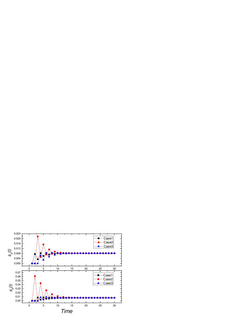
Figure 2: (Color online) The evolution of the strengths of node $a$ and $b$, where nodes $a$ and $b$ are randomly selected for observation. The three cases are in different initial states which simply satisfy $\sum_{i}{s_{i}(0)=1}$. The exponent $\alpha=1$.

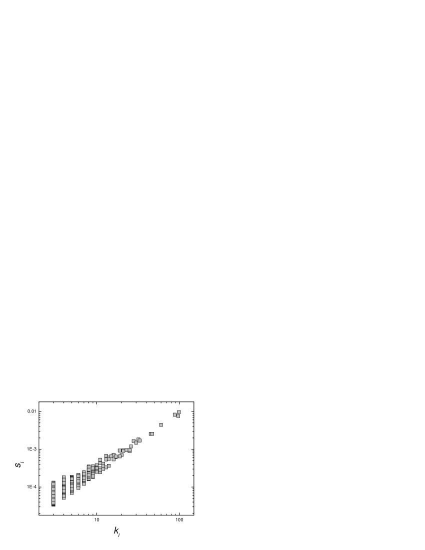
Figure 3: Scatter plots of $s_{i}$ vs $k_{i}$ for all the nodes

III Kinetic equilibrium state

The Eq. 2 can be expressed in terms of a matrix equation, which reads

$$\vec{S}(t+1)=A\vec{S}(t):=\begin{pmatrix}a_{11}&\dots&a_{1n}\\ a_{21}&\dots&a_{2n}\\ {3}\\ a_{n1}&\dots&a_{nn}\\ \end{pmatrix}\cdot\begin{pmatrix}s_{1}(t)\\ s_{2}(t)\\ \dots\\ s_{n}(t)\end{pmatrix}$$ (3)

where the elements of matrix $A$ are given by

$$a_{ij}=\begin{cases}{k^{\alpha}_{i}}/{\sum\limits_{l\in N(j)}k^{\alpha}_{l}}&j\in N(i)\\ 0&\text{otherwise}\end{cases}$$ (4)

Since $\sum\limits_{i=1}^{n}|a_{ij}|=1$, $\forall j$, the spectral radius of matrix $A$ obeys the equality $\rho(A)\leq 1$, according to the Gershgörin disk theorem disk theorem . Here, the spectral radius, $\rho(A)$, of a matrix $A$, is the largest absolute value of an eigenvalue. Further more, since the considered network is symmetry-free (That is to say, the network is strongly connected thus for any two nodes $i$ and $j$, these exists at least one path from $i$ to $j$), $A^{k}$ will converge to a constant matrix for infinite $k$. That is, if given the initial boundary condition to Eq. 3 (e.g. let $\sum\limits_{i=1}^{n}{s_{i}(0)=1}$, where $n$ denotes the total number of nodes in network), then $s_{i}(t)$ will converge in the limit of infinite $t$ as $\lim\limits_{t\rightarrow\infty}s_{i}(t)=s_{i}$ for each node $i$.

Consequently, Denote $\vec{S}:=(\begin{matrix}s_{1},&s_{2}&\dots&s_{n}\end{matrix})^{T}$, one can obtain

$$\vec{S}=A\vec{S}.$$ (5)

That is, for any $i$,

$$s_{i}=\sum\limits_{j\in N(i)}\big{(}{k^{\alpha}_{i}s_{j}}/{\sum\limits_{l\in N(j)}k^{\alpha}_{l}}\big{)}.$$ (6)

From Eq. 5, it is clear that $\vec{S}$ is just the kinetic equilibrium state of the resource flow in our model. Since $\vec{S}=\lim\limits_{k\rightarrow\infty}A^{k}\vec{S}(0)$, $\vec{S}$ is determined only by matrix $A$, if given the initial boundary condition with $\vec{S}(0)$ satisfying $\sum\limits_{i=0}^{n}{s_{i}(0)=1}$. Since matrix $A$ is determined by the topology only, for each node $i$ in the kinetic equilibrium, $s_{i}=\lim\limits_{t\rightarrow\infty}s_{i}(t)$ is completely determined by the network structure. $s_{i}$ denotes the amount of resource eventually allocated to node $i$, thus it is reasonable to define $s_{i}$ as the strength of node $i$.

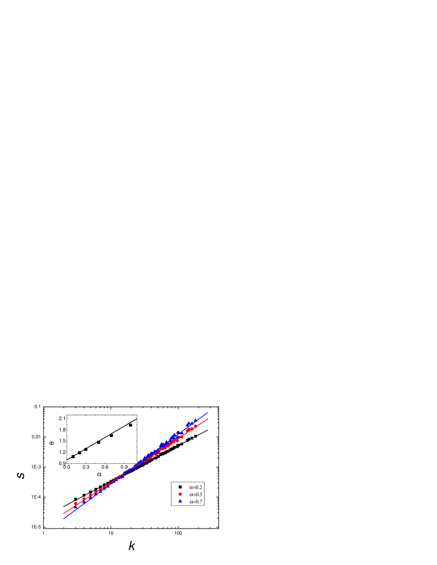
Figure 4: (Color online) The correlation between degree and strength with different $\alpha$. In the inset, the relation between $\theta$ and $\alpha$ is given, where the squares come from the simulations and the solid line represents the theoretical result $\theta=1+\alpha$.

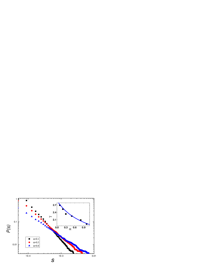
Figure 5: (Color online) The distribution of strength with different $\alpha$. The inset exhibits the relation between $\gamma$ and $\alpha$, where the squares come from the simulations and the solid line represents the theoretic analysis $\gamma=(\alpha+\beta)/(1+\alpha)$.

IV Power-law correlation between strength and degree in scale-free networks

The solution of Eq. (6) reads

$$s_{i}=\lambda k^{\alpha}_{i}\sum\limits_{j\in N(i)}{k^{\alpha}_{j}},$$ (7)

where $\lambda$ is a normalized factor.

In principle, this solution gives the analytical relation between $s_{i}$ and $k_{i}$ when $\sum_{j\in N(i)}{k^{\alpha}_{j}}$ can be analytically obtained from the degree distribution. For uncorrelated networks Newman2002 , statistically speaking we have

$$s_{i}=\lambda k^{1+\alpha}_{i}\sum_{k^{\prime}}P(k^{\prime})k^{\prime\alpha},$$ (8)

where $P(k)$ denotes the probability a randomly selected node is of degree $k$. Since $\lambda\sum_{k^{\prime}}P(k^{\prime})k^{\prime\alpha}$ is a constant when given a network structure, one has $s_{i}\sim k_{i}^{1+\alpha}$, thus

$$s(k)\sim k^{1+\alpha},$$ (9)

where $s(k)$ denotes the average strength over all the nodes with degree $k$.

This power-law correlation $s(k)\sim k^{\theta}$ where $\theta=1+\alpha$, observed in many real weighted networks, can be considered as a result of the conjunct effect of the above power-law correlation and the scale-free property. Obviously, if the degree distribution in a weighted network obeys the form $P(k)\sim k^{-\beta}$, one can immediately obtain the distribution of the strength

$$P(s)\sim s^{-\gamma},$$ (10)

where the power-law exponent $\gamma=(\alpha+\beta)/(1+\alpha)$.

V Simulations

Recent empirical studies in network science show that many real-life networks display the scale-free property Review , thus we use scale-free networks as the samples. Since the Barabási-Albert (BA) model BA is the mostly studied model and lacks structural-biases such as non-zero degree-degree correlation, we use BA network with size $n=5000$ and average degree $\langle k\rangle=6$ for simulations. The dynamics start from a completely random distribution of resource. As is shown in Fig. 2, we randomly pick two nodes $a$ and $b$, and record their strengths vs time $s_{a}(t)$ and $s_{b}(t)$ for three different initial conditions. Clearly, the resource owned by each node will reach a stable state quickly. And no matter how and where the one unit resource flow in, the final state is the same.

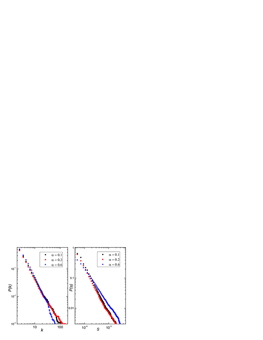
Figure 6: (Color online) The distributions of degree (left panel) and strength (right panel) with different $\alpha$. The networks are generated by the strength-PA mechanism, and those shown here are the sampling of size $n=5000$.

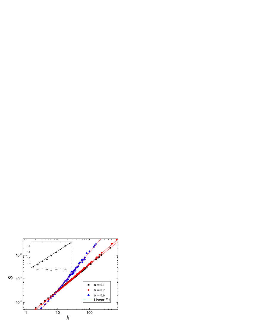
Figure 7: (Color online) The correlation between degree and strength with different $\alpha$. In the inset, the relation between $\theta$ and $\alpha$ is given, where the squares come from the simulations and the solid line represents the theoretical result $\theta=1+\alpha$. The networks are generated by the strength-PA mechanism, and those shown here are the sampling of size $n=5000$.

Similar to the mechanism used to judge the weight of web by Google-searching (see a recent review paper Google about the PageRank Algorithm proposed by Google), the strength of a node is not only determined by its degree, but also by the strengths of its neighbors (see Eq. 7). Although statistically $s(k)\sim k^{1+\alpha}$ for uncorrelated networks, the strengths of the nodes with the same degree may be far different especially for low-degree nodes as exhibited in Fig. 3.

In succession, we average the strengths of nodes with the same degree and plot Fig. 4 to verify our theoretical analysis that there is a power-law correlation $s\sim k^{\theta}$ between strength and degree, with exponent $\theta=1+\alpha$. Fig. 5 shows that the strength also obeys power-law distribution, as observed in many real-life scale-free weighted networks. And the simulations agree well with analytical results.

VI Conclusion remarks

In this paper, we proposed a model for resource-allocation dynamics on scale-free networks, in which the system can approach to a kinetic equilibrium state with power-law strength-degree correlation. If the resource flow is unbiased (i.e. $\alpha=0$), similar to the BBV model Barrat2004b ; Barrat2004c , the strength will be linearly correlated with degree as $s(k)\sim k$. Therefore, the present model suggests that the power-law correlation between degree and strength arises from the mechanism that resources in networks tend to flow to larger nodes rather than smaller ones. This preferential flow has been observed in some real traffic systems. For example, very recently, we investigated the empirical data of Chinese city-airport network, where each node denote a city, and the edge-weight is defined as the number of passengers travelling along this edge per week Liu2006 . We found that the passenger number from one city to its larger-degree neighbor is much larger than that from this city to its smaller-degree neighbor. In addition, in Chinese city-airport network Liu2006 and US airport network Barrat2004a , the power-law exponents are $\theta\approx 1.4$ and $\theta\approx 1.5$, respectively, which is within the range of $\theta$ predicted by the present model.

The readers should be warned that the analytical solution shown in this paper is only valid for static networks without any degree-degree correlation. However, we have done some further simulations about the cases of growing networks (see Appendix A) and correlated networks (see Appendix B). The results are quantitatively the same with slight difference in quantity.

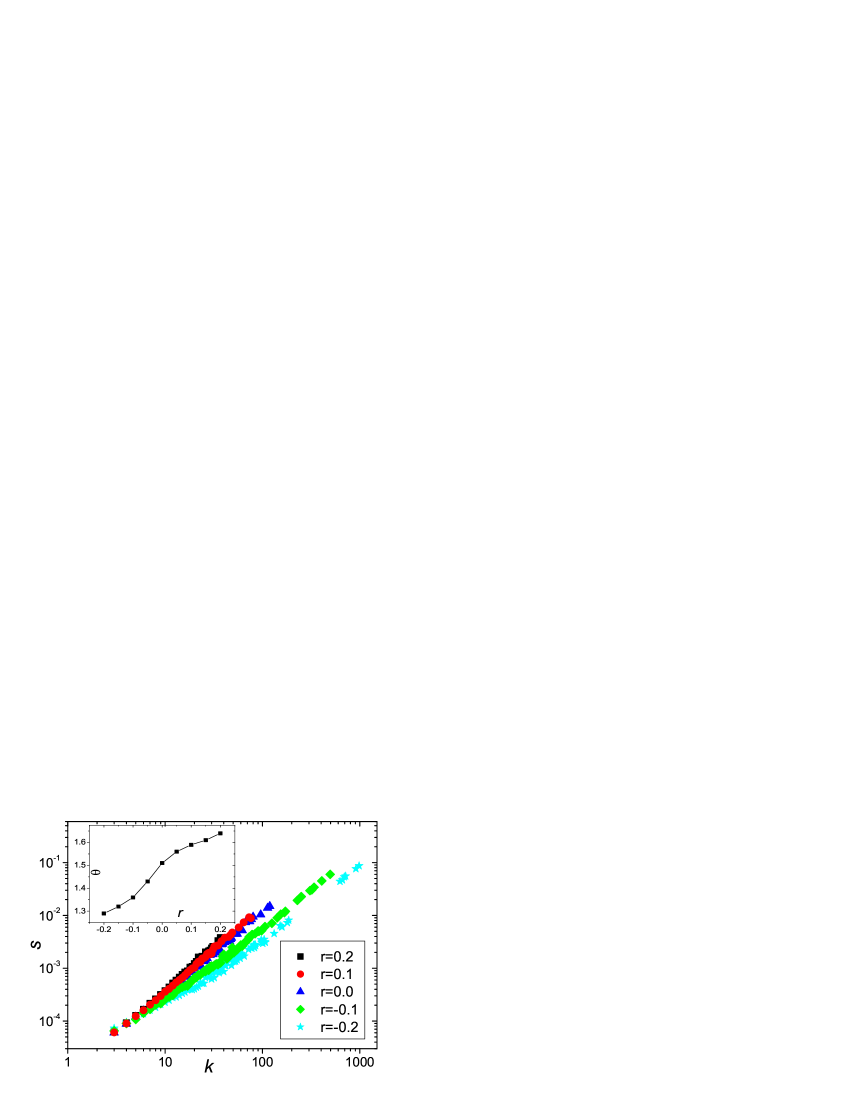
Figure 8: (Color online) The correlation between degree and strength with different assortative coefficients $r$. The parameter $\alpha=0.5$ is fixed. The inset shows the numerically fitting value of $\theta$ vs assortative coefficients. The networks are generated by the generalized BA algorithm GBA1 ; GBA2 of size $n=5000$ and average degree $\langle k\rangle=6$.

Finally, in this model, the resource flow will approach to a kinetic equilibrium, which is determined only by the topology of the networks, so we can predict the weight of a network just from its topology by the equilibrium state. Therefore, our proposed mechanism can well apply to estimate the behaviors in many networks. When given topology of a traffic network, people can easily predict the traffic load in individual nodes and links by using this model, so that this model may be helpful to a better design of traffic networks.

Appendix A The case of growing networks

Since many real networks, such as WWW and Internet, are growing momently. The performance of the present resource-allocation flow on growing networks is thus of interest. We have implemented the present dynamical model on the growing scale-free networks following the usual preferential attachment (PA) scheme of Barabási-Albert BA . Since the topological change is independent of the dynamics taking place on it, and the relaxation time before converging to a kinetic equilibrium state is very short (see Fig. 2), if the network size is large enough (like in this paper $n\sim 10^{3}$), then the continued growth of network has only very slight effect on topology and the results is almost the same as those of the ungrowing case shown above.

Furthermore, we investigate the possible interplay between the growing mechanism and the resource-allocation dynamics. In this case, the initial network is a few fully connected connected nodes, and the resource is distributed to each node randomly. Then, the present resource-allocation process works following Eq. (2), and simultaneously, the network itself grows following a strength-PA mechanism instead of the degree-PA mechanism proposed by BA model. That is to say, at each time step, one node is added into the network with $m$ edges attaching to the existing nodes with probability proportional to their strengths (In a growing BA network, the corresponding probability is proportional to their degrees). Clearly, under this scenarios, there exists strong interplay between network topology and dynamic.

When the network becomes sufficient large ($n\sim 10^{3}$), as shown in Fig. 6, the evolution approaches a stable process with both the degree distribution and strength distribution approximately following the power-law forms. Furthermore, we report the relationship between strength and degree in Fig. 7, which indicate that the power-law scaling, $s(k)\sim k^{\theta}$ with $\theta=1+\alpha$, also holds even for the growing networks with strong interplay with the resource-allocation dynamics.

Appendix B The case of correlated networks

Note that, the Eq. (8) is valid under the assumption that the underlying network is uncorrelated. However, many real-life networks exhibit degree-degree correlation in some extent. In this section, we will investigate the case of correlated networks. The model used in this section is a generalized BA model GBA1 ; GBA2 : Starting from $m_{0}$ fully connected nodes, then, at each time step, a new node is added to the network and $m$ ($<m_{0}$) previously existing nodes are chosen to be connected to it with probability

$$p_{i}\propto\frac{k_{i}+k_{0}}{\sum_{j}(k_{j}+k_{0})},$$ (11)

where $p_{i}$ and $k_{i}$ denote the choosing probability and degree of node $i$, respectively. By varying the free parameter $k_{0}$ $(>-m)$, one can obtain the scale-free networks with different assortative coefficients $r$ (see the Ref. Newman2002 for the definition of assortative coefficient).

The simulation results are shown in Fig. 8, from which one can find that the power-law correlations between strength and degree in the correlated networks are quantitatively the same as that of the uncorrelated networks, however, the power-law exponents, $\theta$, are slightly different. Actually, in the positive correlated networks, the large-degree nodes prefer to connect with some other large-degree nodes rather than those small-degree nodes, thus there may exist a cluster consisting of large-degree nodes that can hold the majority of resource. That cluster makes the large-degree nodes having even more resource than in the uncorrelated case, thus leading to a larger $\theta$. In the inset of Fig. 8, one can find that $\theta$ is larger in the positive correlated networks, and smaller in the negative correlated networks. However, the analytical solution have not yet achieved when taking into account the degree-degree correlation, which needs a in-depth analysis in the future.

References

- (1) W. Li, and X. Cai, Phys. Rev. E 69, 046106 (2004).
- (2) A. Barrat, M. Barthélemy, R. Pastor-Satorras, and A. Vespignani, Proc. Natl. Acad. Sci. U.S.A. 101, 3747 (2004).
- (3) W. -X. Wang, B. -H. Wang, B. Hu, G. Yan, and Q. Ou, Phys. Rev. Lett. 94, 188702 (2005).
- (4) H. -K. Liu, and T. Zhou, Acta Physica Sinica (to be published).
- (5) W. -X. Wang, B. Hu, T. Zhou, B. -H. Wang, and Y. -B. Xie, Phys. Rev. E 72, 046140 (2005).
- (6) M. E. J. Newman, and M. Girvan, Phys. Rev. E 69, 026113 (2004).
- (7) T. Zhou, Z. -Q. Fu, and B. -H. Wang, Prog. Nat. Sci. 16, 452 (2006).
- (8) G. Yan, T. Zhou, J. Wang, Z. -Q. Fu, and B. -H. Wang, Chin. Phys. Lett. 22, 510 (2005).
- (9) A. E. Motter, C. Zhou, and J. Kurths, Phys. Rev. E 71, 016116 (2005).
- (10) M. Chavez, D. -U. Hwang, A. Amann, H. G. E. Hentschel, and S. Boccaletti, Phys. Rev. Lett. 94, 218701 (2005).
- (11) M. Zhao, T. Zhou, and B. -H. Wang, Eur. Phys. J. B (to be published).
- (12) A. Barrat, M. Barthélemy, and A. Vespignani, Phys. Rev. Lett. 92, 228701 (2004).
- (13) A. Barrat, M. Barthélemy, and A. Vespignani, Phys. Rev. E 70, 066149 (2004).
- (14) P. Holme, Adv. Complex Syst. 6, 163 (2003)
- (15) B. Tadić, S. Thurner and G. J. Rodgers, Phys. Rev. E 69, 036102 (2004).
- (16) C. -Y. Yin, B. -H. Wang, W. -X. Wang, T. Zhou, and H. -J. Yang, Phys. Lett. A 351, 220 (2006).
- (17) W. -X. Wang, B. -H. Wang, C. -Y. Yin, Y. -B. Xie, and T. Zhou, Phys. Rev. E 73, 026111 (2006).
- (18) Y. -B. Xie, B. -H. Wang, B. Hu, and T. Zhou, Phys. Rev. E 71, 046135 (2005).
- (19) R. Guimera, S. Mossa, A. Turtschi, and L. A. N. Amaral, Proc. Natl. Acad. Sci. U.S.A. 102, 7794 (2005).
- (20) R. Albert, I. Albert, and G. L. Nakarado, Phys. Rev. E 69, 025103 (2004).
- (21) R. A. Horn, and C. R. Johnson, Matrix Analysis (Cambridge University Press, Cambridge, 1985).
- (22) M. E. J. Newman, Phys. Rev. Lett. 89, 208701 (2002).
- (23) R. Albert, and A. -L. Barabási, Rev. Mod. Phys. 74, 47 (2002).
- (24) A. -L. Barabási, and R. Albert, Science 286, 509 (1999).
- (25) K. Bryan, and T. Leise, SIAM Rev. 48, 569 (2006).
- (26) S. N. Dorogovtsev, J. F. F. Mendes, and A. N. Samukhin, Phys. Rev. Lett. 85, 4633 (2000).
- (27) P. L. Krapivsky, and S. Redner, Phys. Rev. E 63, 066123 (2001).