Early out-of-equilibrium beam-plasma evolution

Abstract

We solve analytically the out-of-equilibrium initial stage that follows the injection of a radially finite electron beam into a plasma at rest and test it against particle-in-cell simulations. For initial large beam edge gradients and not too large beam radius, compared to the electron skin depth, the electron beam is shown to evolve into a ring structure. For low enough transverse temperatures, the filamentation instability eventually proceeds and saturates when transverse isotropy is reached. The analysis accounts for the variety of very recent experimental beam transverse observations.

Beam-plasma interactions have recently received some considerable renewed interest especially in the relatively unexplored regimes of high beam intensities and high plasma densities. One particular motivation lies in the fast ignition schemes (FIS) for inertial confinement fusion Tabak94 . These should involve in their final stage the interaction of an ignition beam composed of MeV electrons laser generated at the critical density surface with a dense plasma target. The exploration of the electron beam transport into the overdense plasma is essential to assess the efficiency of the beam energy deposit. In this matter, transverse beam-plasma instabilities could be particularly deleterious in preventing conditions for burn to be met. Experimental observations recently undertaken in conditions relevant to the FIS have either shown some transverse microscopic filamentation of electron beams Tatarakis03 or some transverse, predominantly macroscopic, beam evolution into a ring structure Koch2002 ; Jung2005 or a superposition of those effects SteinReport2003 ; Jung2005 ; Norreys , with filaments standing out from a ring structure, in a scenario similar to Taguchi et al.’s numerical simulations Taguchi2001 . Weibel instability Weibel is commonly invoked to account for these phenomena, but it is sometimes difficult to find any clear univocal evidence supporting this. Moreover the fact is that, whereas most theoretical and some computational studies are devoted to the linear regime of instabilities originating from current and charge neutralized equilibria, the physics of the fast ignition is intrinsically out-of-equilibrium.

In this Letter, we shall consider the out-of-equilibrium initial value dynamical problem taking place when a radially inhomogeneous electron forward current is launched into a plasma and is still not current compensated. We shall focus on this early stage where collisions may be neglected. Ions will be assumed to form a fixed neutralizing background. In order to simplify both the analysis and the numerical PIC computations, we shall consider the system to be infinite along the beam direction $z$. We shall remove any $z$ dependance by assuming also that plasma density $n_{pe}$ is uniform and constant. At time $t=0$, a relativistic electron beam is switched on in the plasma.

Maxwell equations are linear and can thus be solved for all time to give the electromagnetic fields as functions of the sources, namely beam and plasma current densities, $\mathbf{j}_{b}$ and $\mathbf{j}_{pe}$. We get $\mathop{\rm rot}\nolimits\mathbf{B}=\mu_{0}(\mathbf{j}_{pe}+\mathbf{j}_{b})+1/c^{2}\partial\mathbf{E}/\partial t$ and $\mathop{\rm rot}\nolimits\mathbf{E}=-\partial\mathbf{B}/\partial t$. The electron plasma current $\mathbf{j}_{pe}=-en_{pe}\mathbf{v}_{pe}$ is initially vanishing and may be approximated by linear fluid theory in the initial stage yielding

$$\frac{\partial\mathbf{j}_{pe}}{\partial t}=\varepsilon_{0}\omega_{pe}^{2}\mathbf{E},$$ (1)

with $\omega_{pe}=\sqrt{n_{pe}e^{2}/m_{e}\varepsilon_{0}}$ the plasma pulsation. We Fourier decompose any field $g$ through $g(r,\theta,t)=\sum_{m}g^{(m)}(r,t)\exp\left(im\theta\right)$ and proceed to a Laplace transform in time $\hat{g}^{(m)}\left(r,s\right)=\int_{0}^{\infty}e^{-st}g^{(m)}\left(r,t\right)dt$. Eliminating the electric field components, Maxwell equations in cylindrical geometry yield inhomogeneous wave equations with sources for the magnetic field components. Introducing the operator $\mathcal{L}_{n}[\mu]$ such that

$$\mathcal{L}_{n}[\mu]y\equiv\frac{1}{r}\frac{d}{dr}\left(r\frac{dy}{dr}\right)+\left(\mu^{2}-\frac{n^{2}}{r^{2}}\right)y,$$ (2)

defining $\sigma\equiv\sqrt{s^{2}+\omega_{pe}^{2}}/c$ and neglecting the initial values of the e.m. fields, the wave equations read

$$\text{for }m = 0\text{, }\mathcal{L}_{1}\left[i\sigma\right]\hat{B}_{\theta}^{(0)}=\mu_{0}\frac{\partial\hat{\jmath}_{bz}^{(0)}}{\partial r},$$ (3)

$$\text{for }m \neq 0\text{, }i\mathcal{L}_{m}\left[i\sigma\right]\left(r\hat{B}_{r}^{(m)}\right)=m\mu_{0}\hat{\jmath}_{bz}^{(m)},$$ (4)

with, for any $m$,

$$\mathcal{L}_{m}\left[i\sigma\right]\hat{B}_{z}^{(m)}=\frac{\mu_{0}}{r}\left[im\hat{\jmath}_{br}^{(m)}-\frac{\partial}{\partial r}\left(r\hat{\jmath}_{b\theta}^{(m)}\right)\right].$$ (5)

Let us make the following general statements: Because they are linear, Maxwell equations do not enable spectral changes. If the beam is sufficiently weak, so that the fluid approximation for the bulk plasma remains approximately valid, mode transfers will originate from the beam particles equations of motion. Consequently, if the initial beam is rigorously both rotationally and axially invariant (on $m=0$), it will remain so for all times. Then there are no sources to feed the triad ($B_{r}$, $B_{z}$, $E_{\theta}$) that remains vanishingly small. This is an invitation to focus first on the $m=0$ evolution.

We consider initial beam density and velocity of $n_{b0}(r)=n_{b0}\bar{n}(\tilde{r})$ and $v_{b0z}(r)=v_{b0z}\bar{v}(\tilde{r})$, with $\tilde{r}=r/r_{b}$. Let us introduce here the beam radius $r_{b}$ note1 , the electron skin depth $\lambda_{s}\equiv c/\omega_{pe}$, their ratio $\eta\equiv r_{b}/\lambda_{s}$, and let us define $\alpha=n_{b0}/n_{pe}$, $\beta_{0}=v_{b0z}/c$ and the initial relativistic Lorentz factor $\gamma_{0}=\left(1-v_{b0z}^{2}/c^{2}\right)^{-1/2}=\left(1-\beta_{0}^{2}\bar{v}^{2}\right)^{-1/2}=\gamma_{0}(\tilde{r})$. The Green function $g(r\mid a)$ Duffy solving $\mathcal{L}_{1}\left[i\sigma\right]g=-\delta\left(r-a\right)$ is readily computed as $g(r\mid a)=I_{1}\left(\sigma r^{<}\right)K_{1}\left(\sigma r^{>}\right)$ with $r^{<}=\min(r,a)$ and $r^{>}=\max(r,a)$. The general solution of Eq. (3) is then

$$\hat{B}_{\theta}^{(0)}(r,s)=-\mu_{0}\int_{0}^{+\infty}aI_{1}(\sigma r^{<})K_{1}(\sigma r^{>})\frac{\partial\hat{\jmath}_{bz}^{(0)}}{\partial a}da.$$ (6)

Let us consider the response $\hat{B}_{\theta 1}^{(0)}$ to the initial beam current $j_{b0z}^{(0)}=-en_{b0}v_{b0z}\bar{j}H(t)$ that is switched on at time $0$. Here $H$ denotes the Heaviside step function and $\bar{j}(\tilde{r})=\bar{n}(\tilde{r})\bar{v}(\tilde{r})$. This gives $\hat{\jmath}_{0bz}^{(0)}(\tilde{r},s)=-en_{b0}v_{b0z}\bar{j}(\tilde{r})/s$. Eq. (3) admits then a solution in separate variables. This makes Laplace inversion easier giving

$$\frac{e}{m_{e}}B_{\theta 1}^{(0)}\left(\tilde{r},t\right)=\alpha\beta_{0}\omega_{pe}\eta F(\tilde{r},\eta)\left[1-\cos\left(\omega_{pe}t\right)\right]$$ (7)

where the radial information is contained into

$$F(\tilde{r},\eta)=K_{1}(\eta\tilde{r})\int_{0}^{\tilde{r}}uI_{1}(\eta u)\bar{j}^{\prime}(u)du+I_{1}(\eta\tilde{r})\int_{\tilde{r}}^{\infty}uK_{1}(\eta u)\bar{j}^{\prime}(u)du.$$ (8)

Then, integrating $\partial E_{z}^{(0)}/\partial r=\partial B_{\theta}^{(0)}/\partial t$ and using Eq. (7) immediately gives

$$\frac{e}{m_{e}}E_{z1}^{(0)}\left(\tilde{r},t\right)=\alpha\beta_{0}\eta^{2}c\omega_{pe}\sin\left(\omega_{pe}t\right)\int_{\infty}^{\tilde{r}}F(u,\eta)du.$$ (9)

Finally, the $m=0$ radial electric field component satisfies the wave equation $\partial_{tt}E_{r}^{(0)}+\omega_{pe}^{2}E_{r}^{(0)}=-1/\varepsilon_{0}\partial_{t}j_{br}^{(0)}$. It is easy to check that its initial behavior is given by

$$\frac{e}{m_{e}}E_{r}^{(0)}(r,t)=\alpha\omega_{pe}^{2}\bar{n}(\tilde{r})\int_{0}^{t}\cos\left[\omega_{pe}(t-\tau)\right]v_{b1r}^{(0)}(r,\tau)d\tau.$$ (10)

For the problem under consideration, the beam to plasma density ratio $\alpha$ is typically a small parameter. Eq. (10) will be second order in $\alpha$.

We now wish to compute the beam evolution under the previous self-fields (7), which was ignored in previous studies Kuppers73 . Let us assume that the beam can be treated as a cold fluid and write the $m=0$ fluid equations, dropping the $m=0$ superscripts,

$$\frac{\partial n_{b}}{\partial t}+\frac{1}{r}\frac{\partial}{\partial r}\left(rn_{b}v_{br}\right) = 0,$$ (11)

$$\left(\frac{\partial}{\partial t}+v_{br}\frac{\partial}{\partial r}\right)\left(\gamma v_{br}\right) = -\frac{e}{m_{e}}E_{r}+\frac{e}{m_{e}}v_{bz}B_{\theta},$$ (12)

$$\left(\frac{\partial}{\partial t}+v_{br}\frac{\partial}{\partial r}\right)\left(\gamma v_{bz}\right) = -\frac{e}{m_{e}}E_{z}+\frac{e}{m_{e}}v_{br}B_{\theta}.$$ (13)

Let us write $n_{b}=n_{b0}+n_{b1}(r,t)$, $v_{br}=v_{b1r}(r,t)$ and $v_{bz}=v_{b0z}+v_{b1z}(r,t)$. Considering $\alpha$ as a small parameter, we get a natural hierarchy: first order terms should be of order $\alpha$, second order terms of order $\alpha^{2}$ and so on. Let us explicit first order fluid equations. The radial electric contribution being negligible (10), Eq. (12) gives

$$\gamma_{0}\frac{\partial v_{b1r}}{\partial t}=\alpha\beta_{0}^{2}\eta c\omega_{pe}\bar{v}(\tilde{r})F(\tilde{r},\eta)\left[1-\cos\left(\omega_{pe}t\right)\right]$$ (14)

which yields, using $v_{b1r}(r,t=0)=0$,

$$\beta_{1r}=\frac{v_{b1r}(\tilde{r},t)}{c}=\alpha\eta\beta_{0}^{2}\frac{\bar{v}(\tilde{r})F(\tilde{r},\eta)}{\gamma_{0}(\tilde{r})}\left[\omega_{pe}t-\sin\left(\omega_{pe}t\right)\right].$$ (15)

The first order conservation equation is

$$\frac{\partial n_{b1}}{\partial t}+\frac{1}{r}\frac{\partial}{\partial r}\left(rn_{b0}(r)v_{b1r}\right)=0.$$ (16)

Using (15), this gives, with $n_{b1}(\tilde{r},t=0)=0$,

$$\frac{n_{b1}(\tilde{r},t)}{n_{b0}}=\alpha\beta_{0}^{2}\bar{n}_{1}(\tilde{r})\left(\frac{1}{2}\omega_{pe}^{2}t^{2}+\cos\left(\omega_{pe}t\right)-1\right),$$ (17)

where $\bar{n}_{1}$ is the radial function

$$\bar{n}_{1}(\tilde{r})=-\frac{1}{\tilde{r}}\frac{\partial}{\partial\tilde{r}}\left[\frac{\tilde{r}\bar{j}(\tilde{r})F(\tilde{r},\eta)}{\gamma_{0}(\tilde{r})}\right].$$ (18)

Figure 1: Functions $\bar{n}(\tilde{r})=\left(\tanh\left[2\kappa(1-\tilde{r})\right]+1\right)/2$ and $\bar{n}_{1}(\tilde{r})$ for $\eta=10$ and $\kappa=10$ (bold), $\kappa=5$ (dashed line) and $\kappa=2$ (plain line) for a monokinetic beam.

Eq. (17) shows that $n_{b1}$ has a secular behavior. Thus the present analysis breaks when $n_{b1}/n_{b0}=\mathcal{O}(1)$, namely roughly for $\omega_{pe}t\sim\alpha^{-1/2}$. In order to put this more precisely, we shall study the radial behavior $\bar{n}_{1}$. Let us consider some initially monokinetic beam ($\bar{v}=1$) having density functions of the form

$$\bar{n}(\tilde{r})=\left(\tanh\left[2\kappa(1-\tilde{r})\right]+1\right)/2.$$ (19)

This enables the study of the influence of the beam edge gradients as $\kappa=-\bar{n}^{\prime}(\tilde{r}=1)$. Fig. 1 displays various $\bar{n}$ profiles and their associated first order perturbations $\bar{n}_{1}$. This shows that, within a given initial lapse of time, the natural evolution of the system tends to increase the beam density around some radius below $r_{b}$. This favors the formation of a ring structure for the beam density, that is all the sharper and all the closer to $r_{b}$ that the initial radial beam gradients are high. The emergence of this beam ring formation can be already inferred from the time evolution of test electrons within the azimuthal magnetic self-field corresponding to some given initial profile $\bar{n}$ of the form (19) as shown in Fig. 2. The caustics pattern signals there a cusp formation in the radial beam density. It is important to note that, due to Eq. (6), this behavior is very dependent on the initial beam profile. Indeed, we observed no such caustics pattern nor any visible evolution towards a ring structure for smooth Gaussian initial beam profile, but rather radial focusing prior to the filamentation onset.

Figure 2: Radial trajectories of test electrons for an initial beam profile given by Eq. (19) with $\eta=\kappa=10$.

In order to assess the validity of the first-order analytical results presented above and get an insight into the longer time evolution of the beam-plasma system, we performed particle-in-cell (PIC) simulations using the code CALDER calder in 2-1/2 dimensions $(x,y,v_{x},v_{y},v_{z})$. All species, namely plasma ions and electrons and beam electrons, are described as particles. Beam electrons are injected at $t=0$ in a plasma without current compensation and $\lambda_{s}=0.05$ $\mu$m. Fig. 3 presents the early time evolution of the beam radial and poloidal mean velocities. The initial beam density profile was given by Eq. (19) with $\eta=10$ and $\kappa=2$. The beam was monokinetic with $\gamma_{0}=15$ and $\alpha$ was equal to 0.03. For beam radial velocity, this figure shows a nice agreement with the analytical result (15). As for beam poloidal velocity, it is initially vanishing and its $m=0$ component does remain so. However, poloidal symmetry eventually breaks due to the arising of filamentation instability. This takes place after a short transient during which plasma backcurrent grows. Then the average poloidal velocity start to grow exponentially, with a growth rate that nicely fits the linear filamentation instability one, given by $\gamma_{f}=\beta_{0}\sqrt{\alpha/\gamma_{0}}\omega_{pe}$ Fainberg70 ; BFD05 .

Figure 3: Early time evolution of the modulus of the radial average of the transversal beam velocity ($\beta_{r}=v_{r}/c$ and $\beta_{\theta}=v_{\theta}/c$) in lin-log scale for $\alpha=0.03$ and $\eta=10$, $\kappa=2$ in (19). Beam and plasma transverse temperatures are 1keV.

Fig. 4 presents the longer term evolution of the transverse components of beam velocity for a monokinetic beam with a larger value of $\alpha$ ($\alpha=0.15$) and smaller $\gamma_{0}$ ($\gamma_{0}=3$). As previously, there is an initial phase, between t=0 and $20\omega_{pe}^{-1}$, during which radial velocity grows fast and poloidal velocity remains small. For $\omega_{pe}t\simeq 20$, we can see on the inset of Fig. 4 that beam density presents a clear ring structure at its edge. When the beam current is partially neutralized, filamentation instability starts, breaking the initial azimuthal system symmetry and producing the exponential growth of poloidal beam velocity. When the instability saturates ($\omega_{pe}t\simeq 35$), the magnitudes of both components of the transverse velocity are similar: transverse isotropy is reached. For $\eta$ larger (not shown here), the relative thickness of the initial ring diminishes and once filamentation saturates, the initial structure becomes almost undetectable.

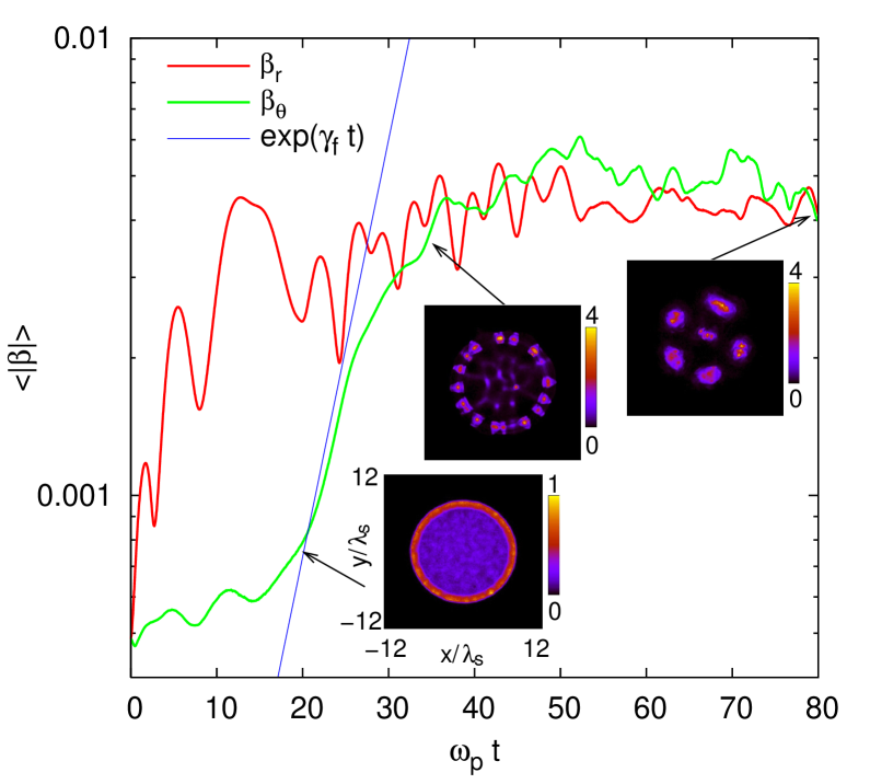
Figure 4: Same as Fig. 3 for $\alpha=0.15$, $\gamma_{0}=3$, $\eta=10$ and $\kappa=20$. Transverse snapshots of beam density are included. Beam and plasma transverse temperatures are 5 keV.

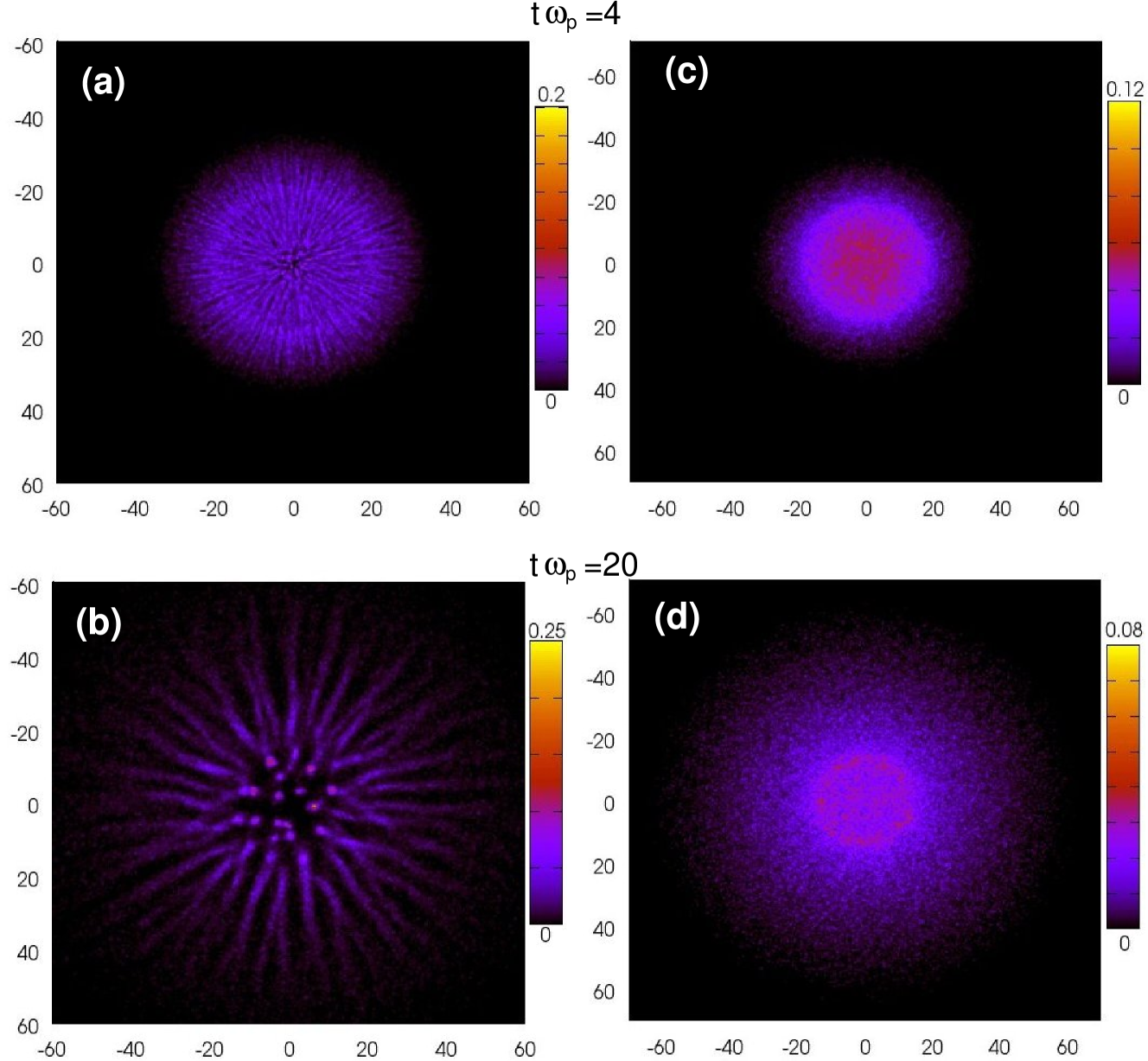
Figure 5: Spatial distribution of the beam density at two times for beams with angular divergence of $15^{\circ}$. Zero emittance (a-b) and large emittance (0.25 $\mu$m) cases (c-d) are shown.

Finally, the evolution changes significantly for beams with finite initial angular divergence. Experimentally, it was found Santos02 that electron beams created by focalizing a laser pulse over a solid target may present divergencies as large as $17^{\circ}$. The origin of these large divergencies is not clear. We performed simulations with beams having an angular divergency of $15^{\circ}$ and two values of emittance. For zero emittance (laminar beam) a dim ring structure appears at short times (Fig. 5(a)), then filamentation takes place (Fig. 5(b)). The large radial velocity produces a fast coalescence of the filaments along the radial direction, resulting in a star-like density pattern. In the high emittance case (Fig. 5(c-d)), no ring structure is apparent. Moreover, the large transverse temperature prevents the onset of the filamentation instability BFD05 ; Silva02 .

In conclusion, our analysis has shown that, depending on its initial radial density and velocity distribution, the shape of an electron beam propagating in a plasma may evolve into a transient ring structure. This results from the natural evolution of the system and not from the usually invoked Weibel instability. If its transverse temperature is low enough, filamentation instability eventually proceeds. The observation of the ring structure is favored by sharp beam edges and not too large beam radius (compared to the electron skin depth). It is not generic which may explain the variety of experimental observations Tatarakis03 ; Koch2002 ; Jung2005 ; SteinReport2003 ; Norreys .

Discussions with A. Bret are gratefully acknowledged.

References

- (1) M. Tabak et al., Phys. Plasmas 1, 1626 (1994).
- (2) M. Tatarakis et al., Phys. Rev. Lett. 90, 175001 (2003).
- (3) J.A. Koch et al., Phys. Rev. E 65, 016410 (2002).
- (4) R. Jung et al., Phys. Rev. Lett. 94, 195001 (2005).
- (5) J. Stein, U. Schramm, D. Habs, E. Fill, J. Meyer-ter-Vehn, and K. Witte, Universität München, Annual Report pp. 63 (2003).
- (6) P. A. Norreys et al., Plasma Phys. Control. Fusion 48, L11 (2006).
- (7) T. Taguchi, T.M. Antonsen, C.S. Liu, and K. Mima, Phys. Rev. Lett. 86, 5055 (2001).
- (8) E.S. Weibel, Phys. Rev. Lett. 2, 83 (1959).
- (9) It would be more rigourous to introduce the rms radius.
- (10) D.G. Duffy, “Green’s Functions with Applications”, Studies in Advanced Mathematics, Chapman & Hall/CRC Ed. (2001).
- (11) G. Küppers, A. Salat, and H.K. Wimmel, Plasma Phys. 15, 429 (1973).
- (12) E. d’Humières, E. Lefebvre, L. Gremillet, and V. Malka, Phys. Plasmas 12, 062704 (2005).
- (13) Ya. B. Faĭnberg, V. D. Shapiro, and V. I. Shevchenko, Sov. Phys. JETP 30, 528 (1970).
- (14) A. Bret, M.-C. Firpo, and C. Deutsch, Phys. Rev. Lett. 94, 115002 (2005); Phys. Rev. E 72, 016403 (2005).
- (15) J.J. Santos et al., Phys. Rev. Lett. 89, 025001 (2002).
- (16) L.O. Silva, R.A. Fonseca, J.W. Tonge, W.B. Mori and J.M. Dawson, Phys. Plasmas 9, 2458 (2002).