Power-law distribution in Japanese racetrack betting

Abstract

Gambling is one of the basic economic activities that humans indulge in. An investigation of gambling activities provides deep insights into the economic actions of people and sheds lights on the study of econophysics. In this paper we present an analysis of the distribution of the final odds of the races organized by the Japan Racing Association. The distribution of the final odds $P_{o}(x)$ indicates a clear power law $P_{o}(x)\propto 1/x$, where $x$ represents the final odds. This power law can be explained on the basis of the assumption that that every bettor bets his money on the horse that appears to be the strongest in a race.

1 Introduction

Since Pascal proposed the theory of probability, the phenomenon of gambling have given inspirations to many mathematicians, physicists and economists. For example, economists have studied gambling activities in order to examine the market efficiency. If bettors try to maximize their expected rewards, it would be equivalent for every race and every horse. In this case, the gambling market is efficient, and there is no assured way to gain money. Gabriel and Marsden studied market efficiency in British racetrack betting and found this gambling market to be inefficient[1]. Russo, Gandar and Zuber conducted a similar study on the National Football League betting market[2]. They found no clear indication of breakdown of efficiency. These results are re-examined Cain et al. and Ioannidis and Peel by different methods[3, 4]

Econophysics and financial engineering are other examples of studies that are closely related to gambling. It is true that gambling and trading differs. Though the stock value is determined by the action of traders, the bettors cannot determine the horse who win the race. However, the trading of stocks bears some similarity to gambling. In trading, traders speculate on stocks, attempt to predict which stock value will rise in the future. This is similar to gambling, in which bettors attempt to predict. Especially, the rewards of winners is determined by the decision of all bettors. This is similar to trading, in which the stock value is determined by the action of traders. Thus, the investigation of gambling will contribute to the advancement of econophysics. In this regards, Park and Domany reported the distribution of odds in Korean horse races[5]. They found the power-law distribution of the final odds. To explain this distribution, they proposed the model of betting, in which the bettors’ estimation of winning probability is affected by the odds.

In this paper, we present an investigation of the distribution of the odds in horse racing in Japan, where national horse races are organized by the Japan Racing Association(JRA). The form of betting in horse race in Japan is same as the one in Korea. There is only one form of betting: pari-mutuel tote bet. In this betting system, the management expenses are deducted from the total amount of the bet, and the winners divide the remaining amount among themselves. In this paper, the odds is defined as the ratio of the reward to the bet. If we neglect the management expenses, the odds of a horse is given as total amount of the bed divided by amount of the bed on the horse.

We show that the distribution of the final odds shows power law $P_{o}(x)\propto x^{-1}$, where $x$ represents the final odds. This is different from the one obtained by Park and Domany, $P_{o}(x)\propto x^{-1.7}$. We propose the model to account for this power-law distribution. One interesting point of this model is that this power-law behavior is obtained by assuming bettors to be irrational. Here the word ‘irrational’ means that bettors do not try to maximize their expected rewards. If we assume bettors to be rational, i. e. attempt to maximize expected rewards, we obtain power-law $P_{o}(x)\propto x^{-2}$, which is different from empirical data.

The outline of this paper is as follows. In the next section, we present the distribution of the final odds in horse races organized by the JRA. We show that the distribution of the final odds $P_{o}(x)$ and that of winners’ odds $P_{w}(x)$ exhibit power-law behaviors, $P_{o}(x)\propto x^{-1}$ and $P_{w}(x)\propto x^{-2}$. In section 3, we propose the model to account for this power-law distribution. In section 4, we make some discussion on our results.

2 Investigation of the final odds in racing organized by the JRA

We analyze the data of 1750 races organized by the JRA between February and July 2005. A total of 24493 horses participated in these races. For simplicity, we investigate only the odds of the win bets, without considering other bets such as dual forecasts or place bets.

In Fig.1, we plot the distribution of the final odds $P_{o}(x)$ for each month, where $x$ represents the final odds. It should be noted that this distribution is not one of the winning payouts; this figure shows the distribution of the final odds, including the losers’ odds. The distribution $P_{o}(x)$ for each month is very similar. At $x<100$, $P_{o}(x)$ follows the power-law distribution, $P_{o}(x)\propto x^{-\gamma}$, and decays exponentially at $x>100$. In order to obtain a clearer picture of the power-law distribution, we plot the total half-year distribution in Fig.2. This data indicates that $\gamma\sim 1$. The distribution of the final winners’ odds is also interesting. In the same figure, we also plot the half-year distribution of winners’ odds. This data shows that the distribution of the winning payouts also follows the power law, $P_{w}(x)\propto 1/x^{2}$.

It should be noticed that these data appear to be consistent with the efficiency of the gambling market. We assume that we bet on a horse whose final odds are represented by $x$. Then, the probability that the horse win is proportional to $P_{w}(x)/P_{o}(x)$. Because the expected reward is represented by $xP_{w}(x)/P_{o}(x)$, the empirical data shows that $P_{w}(x)/P_{o}(x)$ is proportional to $x$ and that the expected reward is independent of $x$.

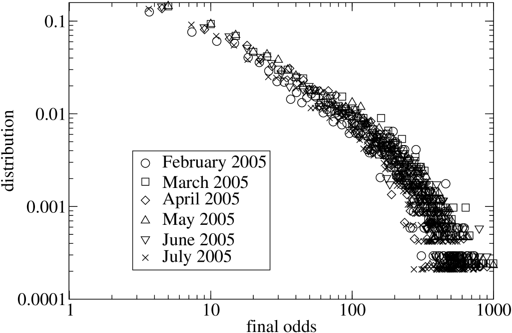
Figure 1: Distribution of the final odds between February and July 2005.

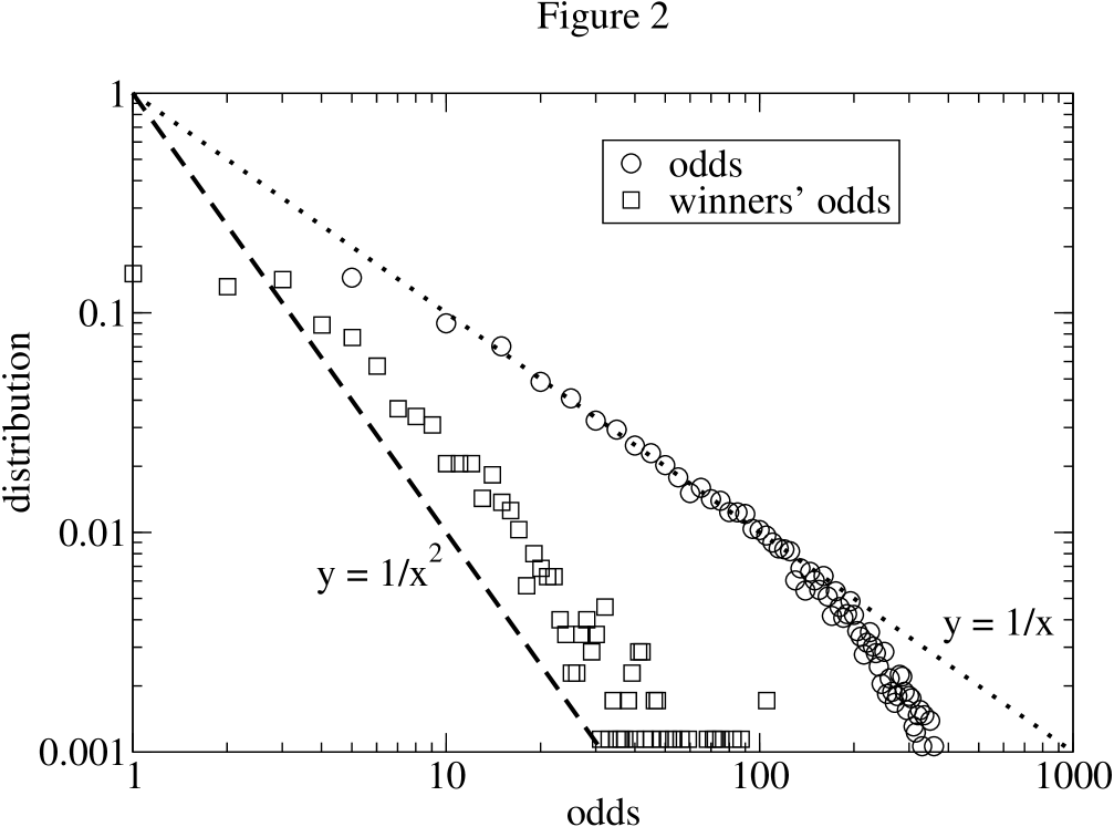
Figure 2: Total distribution of the odds and the winners’ odds between February and July 2005.

However, the efficiency of the gambling market does not mean the rationality of bettors. If bettors are rational, they will bet on the horse whose expected rewards is maximum, and the expected rewards will become equivalent for all horses. It is true that rationality of bettors is a sufficient condition for the efficient market, however, it is not a necessary condition. It should also be noted that the power-law distribution of the final odds cannot be explained solely by the rationality of bettors. We will need some other assumptions to explain the distribution. In the next section, we propose a model to account for these power-law distributions of the final odds.

3 Model simulation

In this section, we propose a model to account for the distribution of the final odds. In order to construct the model, we must focus on the following points. First, the strength of each horse running in a race varies. One horse may be stronger than the other horses, and the weakest horse may perhaps lose the race. Therefore, we must include the differences in the strengths of horses in the model. Second, the strength of each horse provides the probability of winning. Even the strongest horse can lose the race if he is in poor health. Therefore, it appears natural to assume that the probability of winning is given by a function of the strength of the horse. Third, bettors are unaware of the exact strength of the horses. While they do know that some horses are stronger than the others, they do not know the exact strength and cannot precisely estimate the probability of winning.

Considering these points, we propose the following model:

(1)

Each horse running in a race has a parameter called ‘strength’ $s$, $0<s\leq 1$. $s_{i}$, the strength of horse $i$, is given by a uniform random number between 0 and 1.

(2)

Each bettor estimates the strength of horse $i$ as $s_{i}+r_{i}$, where $r_{i}$ is the Gaussian random number. $r_{i}$ varies for each bettor, and the strength estimated by each bettor also differs.

(3)

Each bettor bets his money on the horse that appears to have the maximum strength in a race. As observed, bettors do not know the exact strength of the horses. They place their bets under incorrect estimation of the strength given by the previous rule. For simplicity, we assume that every bettor bets the same amount of money.

(4)

After each betting, $x_{i}$, the odds of a horse $i$, is updated as $x_{i}=n_{tot}/n_{i}$, where $n_{tot}$ and $n_{i}$ represents the total number of bettors and number of bettors who bets on horse $i$, respectively. This rule means that we neglect the management expenses, and the total amount of bets is divided among the winners. This simplification does not lead to any problems.

(5)

The winning probability of a horse is proportional to his strength.

This model has three parameters. The first parameter is the number of horses that participate in one race. Although the number of horses differs with each race, in the following simulation, we assume that 14 horses participate in one race. This approximates the average number of horses participate in one race, 13.996. The second parameter is the number of bettors. We set this number as 10000. The qualitative result of this simulation does not depend on the details of this parameter, if it is sufficiently large. The third parameter is $\sigma$, the dispersion of a random number $r_{i}$. In our model, $\sigma$ is the only parameter we should adjust for fitting.

To see the $\sigma$-dependence of the distribution of the final odds, we plot the distribution $P_{o}(x)$ obtained by our model for some typical $\sigma$ in Fig.3. If $\sigma\ll 1$, almost all bettors bet on the strongest horse, and $P_{o}(x)$ shows sharp peak at $x=1$. On the other hand, if $\sigma\gg 1$ the strength of horse scarcely affects the choice of bettors. Every bettor bets on the horse almost at random, and $P_{o}$ will show sharp peak at $x=h_{tot}$, where $h_{tot}$ is the total number of horses. The results of simulation at $\sigma=0.05$ and $\sigma=5.0$ shown in Fig.3 are consistent with this qualitative discussion. Though the region where $P(x)\propto 1/x$ appears in both cases, these results do not qualitatively coincide with empirical data. In the following of this paper, we use $\sigma=0.5$ and compare the empirical data and the result of simulation.

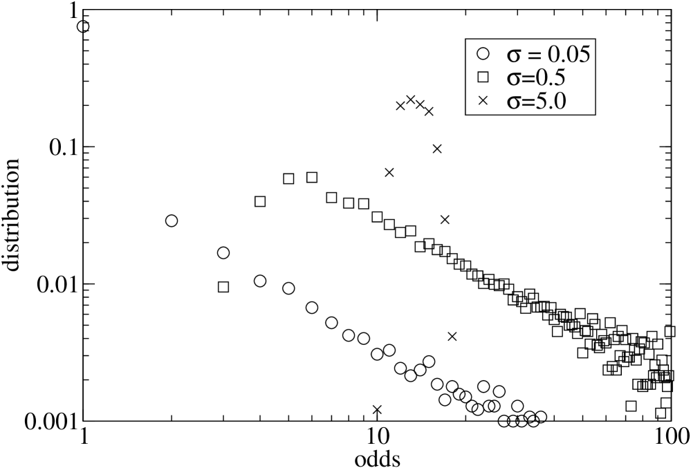
Figure 3: Distribution obtained from our model at $\sigma=0.05$, $0.5$ and $5.0$. Each distribution is obtained by simulating our model 1000 times.

We calculate the distribution of the final odds at $\sigma=0.5$ by simulating this model 10000 times. The results of the simulation are shown in Figs. 4 and 5. With regard to the distribution of the final odds shown in Fig.4, both the power-law behavior at $x<100$ and the exponential decay at $x>100$ are reproduced well in our model and are represented by squares. On the other hand, the power-law behavior of the distribution of the winners’ odds shown in Fig.5 is also reproduced by the simulation, although the absolute value differs slightly. These results suggest the validity of our model.

However, the economists who believe in the rationality of people will expect that the bettors attempt to maximize their expected returns. If this is true, the bettors bet their money on the horse whose expected rewards (winning probability multiplied by odds) is maximum, instead of betting on the one whose probability of winning is maximum. However, the simulation shows that the empirical data cannot be accounted for by using the ‘maximize the expected rewards’ model. In the ‘maximize the expected rewards’ model, we use the following rule instead of the rule (3) in our model:

(3’)

Each bettor bets his money on the horse that appears to have the maximum expected rewards in a race. Because the probability that a horse wins is proportional to his strength, the expected reward of horse $i$ seems proportional to $(n_{tot}+1)(s_{i}+r_{i})/(n_{i}+1)$. Bettors bets his money on the horse $i$ that seems to have maximum expected reward.

Here we note that the expected rewards is not $n_{tot}(s_{i}+r_{i})/n_{i}$, because if the bettor bets on the horse $i$, the odds of the horse changes from $n_{tot}/n_{i}$ to $(n_{tot}+1)/(n_{i}+1)$. In this model, the distribution of the odds is not $\delta$-function even if $r_{i}=0$, because bettors bet on the weak horse with high odds. If the number of bettors is large enough, the expected rewards $x_{i}s_{i}$ will be same for all horses. The result of the simulation based on this model is indicated by the cross in Figs. 4 and 5. In this ‘maximize the expected rewards’ calculation, we take $\sigma=0.001$. In this model, the distribution of the final odds $P_{o}(x)$ and winners’ odds $P_{w}(x)$ are approximately proportional to $1/x^{2}$ and $1/x^{3}$, respectively. These results are inconsistent with the empirical data.

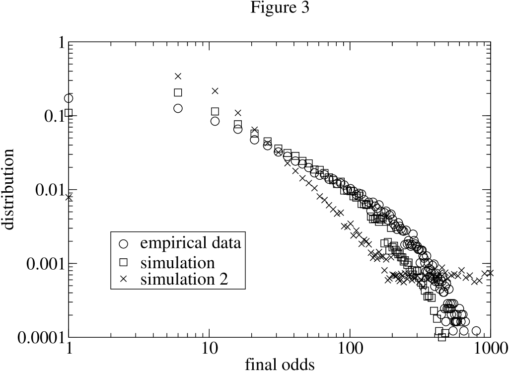
Figure 4: Comparison of the empirical distribution of the final odds and model calculation. Circles, squares and crosses represent the empirical data, the result of the model simulation and the result of the model simulation in which bettors attempt to maximize their expected rewards, respectively.

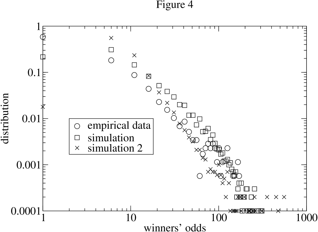
Figure 5: Comparison between the empirical distribution of the winners’ odds and model calculation. Circles, squares and crosses represent the empirical data, the result of the model simulation, and the result of the model simulation in which bettors attempt to maximize their expected rewards, respectively.

4 Conclusion and Discussion

We investigate the distribution of the final odds in horse races organized by the JRA. The distribution of the final odds shows the clear power-law $P_{o}(x)\propto x^{-1}$ at $x<100$. The distribution of the winners’ odds also shows a power-law behavior, $P_{w}(x)\propto x^{-2}$. In order to explain these distributions, we propose a model for the action of bettors. Numerical simulation of this model shows good agreement with the observation.

These results show that the actions of the bettors in gambling can be described by our simple model. In particular, it should be noted that our model does not consider the bettors to be rational. In economics, a rational person will attempt to maximize his expected rewards and bet on the horse whose expected rewards appear to be maximum. In the usual model of the efficient market, the efficiency is guaranteed by this rationality. On the other hand, in our model bettors bet on the horse whose winning probability is maximum. Bettors do not bet on the weak horse, even if the odds are extremely high. Of course, we may be able to make the model to explain the distribution of odds, assuming rational bettors. For example, the different distribution of strength of horses $s_{i}$ will give the different distribution of the final odds. However, such a model will be more complicated one than our model. Therefore it seems natural to conclude that bettors are irrational in horse-racing.

The inconsistency between our investigation and that of Park et al.[5] is also interesting. They studied the odds in Korean horse races and found the power-law distribution of the final odds, $P_{o}(x)\propto x^{-1.7}$. To explain this power-law distribution, the assumed that bettors overestimate the probability of winning of the horse whose odds is small. Due to this effect, bettors overestimate the winning probability of strong horse. Both of their empirical data and simulation model are different from ours. In Japanese horse races, the distribution of odds shows different power-law, $P_{o}(x)\propto x^{-1}$. One of the possible origin of this difference is the difference in the distribution of the strength of horse. As we noticed, the different distribution of the strength of horses will give the different distribution of the final odds. However, it will be difficult to obtain the distribution of the strength from empirical data. We also note that the model of Parks et al. cannot explain our empirical data even if the distribution of strength is changed. As noticed above, their model assumes that the winning probabilities of strong horses are overestimated. If it is true, we can obtain larger expected rewards when we bet on the horse with large odds. However, our data show that the expected rewards is almost independent from odds.

Our paper will shed light on the understanding of other economic activities of people, such as those in the financial market. The dynamics of the financial market is one of the main concern in econophysics. In this regards, the understanding of the action of traders plays the crucial role. If we know the action of each trader, we can make a reliable model to emulate the market. In this paper, we construct a model of bettors in gambling market, which can explain the distribution of the final odds very well. The knowledge obtained from the study of gambling market will give important information to the understanding of the financial market.

References

- [1] P. E. Gabriel and J. R. Marsden, The Journal of Political Economy 98 (1990) 874.
- [2] B. Russo, J. M. Gandar, and R. A. Zuber. Market rationality tests based cross-equation restrictions. Journal of Monetary Economics, 24 (1989) 455.
- [3] M. Cain, D. Law, and D. Peel, Journal of Forecasting, 19 (2000) 575.
- [4] C. Ioannidis and D. Peel, Economics Letters, 87 (2005) 221.
- [5] K. Park and E. Domany, Europhysics Letters, 53 (2001) 419.