Deep-water internal solitary waves near critical density ratio

Abstract

Bifurcations of solitary waves propagating along the interface between two ideal fluids are considered. The study is based on a Hamiltonian approach. It concentrates on values of the density ratio close to a critical one, where the supercritical bifurcation changes to the subcritical one. As the solitary wave velocity approaches the minimum phase velocity of linear interfacial waves (the bifurcation point), the solitary wave solutions transform into envelope solitons. In order to describe their behavior and bifurcations, a generalized nonlinear Schrödinger equation describing the behavior of solitons and their bifurcations is derived. In comparison with the classical NLS equation this equation takes into account three additional nonlinear terms: the so-called Lifshitz term responsible for pulse steepening, a nonlocal term analogous to that first found by Dysthe for gravity waves and the six-wave interaction term. We study both analytically and numerically two solitary wave families of this equation for values of the density ratio $\rho$ that are both above and below the critical density ratio $\rho_{cr}$. For $\rho>\rho_{cr}$, the soliton solution can be found explicitly at the bifurcation point. The maximum amplitude of such a soliton is proportional to $\sqrt{\rho-\rho_{cr}}$, and at large distances the soliton amplitude decays algebraically. A stability analysis shows that solitons below the critical ratio are stable in the Lyapunov sense in the wide range of soliton parameters. Above the critical density ratio solitons are shown to be unstable with respect to finite perturbations.

PACS: 05.45.Yv; 47.55.-t; 47.90.+a

I Introduction

The main goal of this paper is to study bifurcations for one-dimensional internal solitary waves propagating along the interface between two ideal fluids with different densities $\rho_{1}$ and $\rho_{2}$. The lighter fluid with density $\rho_{2}$ lies above the heavier fluid with density $\rho_{1}$: $\rho=\rho_{2}/\rho_{1}<1$. These bifurcations occur if the solitary wave velocity $V$ coincides with the minimum phase velocity $V_{cr}$ of linear internal waves. If the upper density $\rho_{2}$ is small enough compared to the lower density $\rho_{1}$, then a bifurcation similar to that for pure gravity-capillary waves occurs [1, 2, 3, 4]. In this case solitary waves undergo a supercritical bifurcation at the critical velocity: their form approaches the form of the envelope solitons for the focusing one-dimensional nonlinear Schrödinger equation (1D NLSE) [5, 6]. The soliton amplitude behaves universally near the critical velocity $V=V_{cr}$: it vanishes like $(V_{cr}-V)^{1/2}$. The width of the solitary wave increases proportionally to $(V_{cr}-V)^{-1/2}$.

As the density ratio $\rho$ increases, the character of the nonlinear interactions changes. The four-wave coupling coefficient decreases and vanishes at $\rho=\rho_{cr}=(21-8\sqrt{5})/11$ [7], that is when $\rho\approx 0.283$. Such a value may not be obtained easily in a two-fluid configuration. However, it may be relevant in a three-layer (or more) configuration [8], or in nonlinear optics, where similar singularities can occur. Above the critical ratio, solitary waves undergo a subcritical bifurcation: at the critical velocity, their amplitude jumps from zero for $\rho$ below $\rho_{cr}$, up to finite values when $\rho$ is above the critical density ratio. In order to describe such type of bifurcation, it is necessary to keep the next order terms beyond the classical 1D NLSE. When the density ratio varies in a neighborhood of the critical density ratio, it is possible to use, as in the derivation of the classical NLSE, perturbation theory assuming that the interacting wave amplitudes are small. At leading order, one needs to keep three kinds of terms. The first one, coming from the four-wave interaction, takes into account the so-called Lifshitz invariant [9]. This term is local relative to the amplitude of the soliton and its first spatial derivative and, as was shown in [10], appears from the expansion of four-wave interaction element under the assumption about its analytical dependence. However, for deep-water internal waves, as we show in this paper, there exists also a nonlocal term which has the same order of magnitude as the first one [11]. Its structure is similar to the Dysthe term first found for water (gravity) waves [12] (see also [13]). In the case of water waves, this term is responsible for the interaction of a narrow wave packet (in $k$-space) with mean flow, induced by the packet. The third term takes into account six-wave interactions. In order to find the six-wave coupling coefficient, one needs to calculate all possible renormalizations due to three-, four- and five-wave interactions and therefore this partial problem requires a lot of cumbersome calculations. For these calculations we use the Hamiltonian formalism (see the review [14], as well as the papers [15, 10]), which appears to be the most adequate method for this subject. In [7], a different method was used: the problem was reformulated as a spatial dynamical system and only the reversibility was exploited. It is necessary to underline also that the use of the Hamiltonian approach to study solitary waves gives an appropriate framework for the temporal behavior of the dynamics of solitary waves, e.g. their stability. Through this formalism, it is easy to perform different kinds of averaging and perturbations. Second, it is crucial that by applying the Hamiltonian technique the averaging equations of motion retain their original Hamiltonian form. In particular, this is of great help for the investigation of soliton stability (see, for instance, [10]).

II Basic equations

Consider the interface $z=\eta(x,t)$ between two ideal incompressible fluids with respective densities $\rho_{1}$ and $\rho_{2}$, in the presence of gravity (with the acceleration $g$ acting down the vertical $z-$axis) and capillarity with interfacial tension $\sigma$. We shall assume that the lighter fluid with density $\rho_{2}$ occupies the region $\infty>z>\eta(x,t)$, and respectively the heavier fluid occupies the region $-\infty<z<\eta(x,t)$. Flows of both fluids are considered to be potential and two-dimensional. The fluid velocities are given by

$\displaystyle\mathbf{v}_{1,2}=\nabla\phi_{1,2},$

where the velocity potentials $\phi_{1}$ and $\phi_{2}$ satisfy Laplace’s equation

$$\Delta\phi_{1,2}=0.$$ (II.1)

These equations are subject to the following boundary conditions. Far from the interface as $z\to\pm\infty$

$\displaystyle\phi_{1,2}\to 0.$

On the interface $z=\eta(x,t)$ the kinematic conditions hold:

$$\frac{\partial\eta}{\partial t}=(-v_{x}\eta_{x}+v_{z})_{1,2}.$$ (II.2)

The dynamic condition reduces to the discontinuity of pressures across the interface due to capillarity:

$\displaystyle p_{1}-p_{2}=-\sigma\frac{\partial}{\partial x}\left(\frac{\eta_{x}}{\sqrt{\eta_{x}^{2}+1}}\right).$

The use of Bernoulli equations in each fluid allows to rewrite the latter equation in terms of potentials and their derivatives:

$$\rho_{1}\left(\frac{\partial\phi_{2}}{\partial t}+\frac{1}{2}(\nabla\phi_{2})^{2}+g\eta\right)-\rho_{2}\left(\frac{\partial\phi_{1}}{\partial t}+\frac{1}{2}(\nabla\phi_{1})^{2}+g\eta\right)=\sigma\frac{\partial}{\partial x}\left(\frac{\eta_{x}}{\sqrt{\eta_{x}^{2}+1}}\right).$$ (II.3)

The equations (II.1)–(II.3) conserve the total energy:

$$H=K+U,$$ (II.4)

where the kinetic energy is equal to

$\displaystyle K=\int_{z>\eta}\frac{\rho_{2}(\nabla\phi_{2})^{2}}{2}\;d\mathbf{r}+\int_{z<\eta}\frac{\rho_{1}(\nabla\phi_{1})^{2}}{2}\;d\mathbf{r}$

and the potential energy is given by the expression

$\displaystyle U=\int(\rho_{1}-\rho_{2})\frac{g\eta^{2}}{2}\;dx+\int\sigma\left(\sqrt{\eta_{x}^{2}+1}-1\right)\;dx.$

As shown first in [16] (see also [17, 18, 14, 19]), the equations of motion (II.2) and (II.3) together with the Laplace equations (II.1) represent a Hamiltonian system. The Hamiltonian coincides with the energy (II.4). The new variables $\Psi=(\rho_{1}\psi_{1}-\rho_{2}\psi_{2})$ and the interface shape $\eta$ are canonical conjugate variables:

$$\frac{\partial\eta}{\partial t}=\frac{\delta H}{\delta\Psi},\vskip 3.0pt plus 1.0pt minus 1.0pt\ \ \frac{\partial\Psi}{\partial t}=-\frac{\delta H}{\delta\eta},$$ (II.5)

where $\psi_{1,2}=\phi_{1,2}|_{z=\eta}$. The given Hamiltonian form generalizes Zakharov’s canonical form for free-surface hydrodynamics [20]. A Hamiltonian formulation of the problem of a free interface between two ideal fluids, under rigid lid boundary conditions for the upper fluid, was also given by Benjamin & Bridges [21]. Craig & Groves [22] give a similar expression, by using the Dirichlet-Neumann operators for both the upper and lower fluid domains (see also [23]).

The Hamiltonian can be expanded in series with respect to powers of the canonical variables. In this case the steepness of the interface plays the role of a small parameter of expansion. Due to the conservation of the total mass for each fluid this expansion begins with the quadratic term.

It is more convenient to work in Fourier space. Let us introduce the normal variables $a_{k}$ by means of the following formulas:

$$\Psi(k)=i\sqrt{\frac{(1+\rho)\omega_{k}}{2|k|}}(a_{k}-a^{*}_{-k}),$$ (II.6)

$$\eta(k)=\sqrt{\frac{|k|}{2(1+\rho)\omega_{k}}}(a_{k}+a^{*}_{-k}),$$ (II.7)

where the density $\rho_{1}$ is set equal to unity and $\rho_{2}=\rho$. In these formulas

$$\omega_{k}=\left(\frac{|k|}{1+\rho}[g(1-\rho)+\sigma k^{2}]\right)^{1/2}$$ (II.8)

is the dispersion relation for linear internal waves and $k$ is the wave vector directed along the $x-$axis (1D case).

The transformation (II.6) diagonalizes the quadratic part of the Hamiltonian,

$\displaystyle H_{0}=\int\omega_{k}|a_{k}|^{2}dk.$

As a result, the equations of motion in the new variables $a_{k}$ take the standard form [14]:

$$\frac{\partial a_{k}}{\partial t}=-i\frac{\delta H}{\delta a^{*}_{k}},$$ (II.9)

with the Hamiltonian

$\displaystyle H=H_{0}+H_{\mathrm{int}},$

where $H_{\mathrm{int}}$ is responsible for the nonlinear interactions between waves. In the given case of internal waves the expansion of $H_{\mathrm{int}}$ in the wave amplitude will contain powers starting with the cubic terms.

Consider a solution of Eq. (II.9) in the form of a solitary wave propagating with constant velocity $V$. Then the potentials and the shape $\eta$ of the interface will depend on $x$ and $t$ through the combination $x-Vt$. In particular, the inverse Fourier transform of $a_{k}$,

$\displaystyle\psi(x,t)=\frac{1}{\sqrt{2\pi}}\int a_{k}(t)e^{ikx}dk,$

will be a function of $(x-Vt)$ only.

In Fourier space such dependence implies an exponential dependence in time for the normal variables:

$\displaystyle a_{k}(t)=c_{k}e^{-ikVt},$

where the time-independent amplitude $c_{k}$ is defined from the equation

$$(\omega_{k}-kV)\,c_{k}=-\frac{\delta H_{\mathrm{int}}}{\delta c_{k}^{*}}\equiv f_{k}.$$ (II.10)

This equation can be casted into the following variational problem:

$$\delta(H-VP)=0,$$ (II.11)

where $P=\int k|c_{k}|^{2}dk$ is the total momentum of the wave system. This means that a solution to this equation represents a stationary point of the Hamiltonian $H$ for fixed momentum $P$.

A solution to Eq. (II.10) in the form of a solitary wave is possible if the difference $\omega_{k}-kV$ is sign-definite. When the equation

$$\omega_{k}=kV$$ (II.12)

has real roots (say $k=k_{0}$), then, in accordance with $x\delta(x)=0$, the solution of (II.10) will be of the form:

$\displaystyle c_{k}=A_{1}\delta(k-k_{0})+\frac{f_{k}}{\omega_{k}-kV},\quad f_{k_{0}}=0.$

Hence taking the first term as the zero approximation, after iteration the solution of this equation can be represented as an infinite series with respect to $\delta(k-nk_{0})$:

$\displaystyle c_{k}=\sum_{n}A_{n}\delta(k-nk_{0}).$

In $x-$space, this solution is equivalent to a periodic solution (for details, see [10, 15]). Physically, this criterion is very transparent. The equality (II.12) is the resonance condition for Cherenkov radiation of waves by an object moving with the velocity $V$. Due to such radiation a solitary wave will lose its energy and therefore cannot be steady.

For the internal wave dispersion (II.8) the maximum solitary wave velocity $V$ coincides with the minimum phase velocity of linear waves:

$\displaystyle V_{cr}=\min\,\frac{\omega_{k}}{k}.$

It occurs when

$$k=k_{0}=\left[\frac{g(1-\rho)}{\sigma}\right]^{1/2}.$$ (II.13)

At this point the values of the linear frequency and critical velocity are

$$\omega_{0}\equiv\omega(k_{0})=\sqrt{2Agk_{0}}\quad\mbox{ and }\quad V_{cr}\equiv\frac{\omega_{0}}{k_{0}}=\sqrt{\frac{2Ag}{k_{0}}},$$ (II.14)

where

$\displaystyle A=\frac{1-\rho}{1+\rho}$

is the Atwood number.

As the maximum solitary wave velocity is approached, the amplitude $c_{k}$ given by (II.10) reaches a very sharp maximum at the point $k=k_{0}$, where the straight line $\omega=kV$ touches the dispersion curve $\omega=\omega_{k}$:

$$c_{k}=\left[\frac{1}{2}\omega^{\prime\prime}\kappa^{2}+k_{0}(V_{cr}-V)\right]^{-1}f_{k}.$$ (II.15)

Here $\kappa=k-k_{0}$ and $\omega^{\prime\prime}=\partial^{2}\omega/\partial k^{2}$ is the positive-definite second derivative of $\omega_{k}$ taken at $k=k_{0}$: $\omega^{\prime\prime}=\omega_{0}/(2k_{0}^{2})>0$. Hence one can see that as $V\to V_{cr}$ the width of the distribution $\Delta k$ tends to zero, which corresponds to the peak at $k=k_{0}$ becoming narrower and narrower. Due to the nonlinearities of the wave system this peak generates multiple harmonics near $k=nk_{0}$ with integer $n$. If the amplitude of this peak is small (if, for instance, it vanishes smoothly while approaching the critical velocity) then we can use the perturbation theory that consists in expanding $\psi$ through its harmonics:

$$\psi({x^{\prime}})=\sum_{n=-\infty}^{\infty}\psi_{n}(X)e^{ink_{0}x^{\prime}},\quad x^{\prime}=x-Vt.$$ (II.16)

Here the small parameter

$$\lambda=\sqrt{1-V/V_{cr}}$$ (II.17)

and the “slow” coordinate $X=\lambda x^{\prime}$ are introduced, so that $\psi_{n}(X)$ is the amplitude of the envelope of n-th harmonic. The assumption that the solitary wave amplitude vanishes continuously at $V=V_{cr}$ means that the leading term of the series in Eq. (II.16) corresponds to the first harmonic, and all other harmonics are small with respect to the parameter $\lambda$. This is the condition under which the nonlinear Schrödinger equation is derived (see, for example, [15, 24, 25]). In this case, at leading order in $\lambda$, we obtain the stationary NLSE (compare with [15, 10, 26])

$$-\lambda^{2}\omega_{0}\psi_{1}+\frac{\omega_{0}}{4k_{0}^{2}}\frac{\partial^{2}\psi_{1}}{\partial x^{2}}-\mu|\psi_{1}|^{2}\psi_{1}=0,$$ (II.18)

where $\mu$ is related to the matrix element $\widetilde{T}_{k_{0}k_{1}k_{2}k_{3}}$ of four-wave interactions (see below) as

$$\mu=2\pi\widetilde{T}_{k_{0}k_{0}k_{0}k_{0}}.$$ (II.19)

¿From now on, we drop the subscript $1$ for $\psi_{1}$. In complete correspondence with (II.11), the envelope equation (II.18) can be recasted in the following variational problem:

$$\delta(\overline{H}+\omega_{0}\lambda^{2}N)=0,$$ (II.20)

where

$\displaystyle N=\int|\psi|^{2}\,dx$

is the number of waves or the wave action. The (averaged) Hamiltonian $\overline{H}$ is given by the expression

$\displaystyle\overline{H}=\frac{1}{2}\int\omega^{\prime\prime}|\psi_{x}|^{2}\;dx+H_{\mathrm{int}}^{(4)}.$

In this approximation the leading term in the interaction Hamiltonian $H_{\mathrm{int}}$ has the form

$$H_{\mathrm{int}}^{(4)}=\frac{\widetilde{T}_{k_{0}k_{0}k_{0}k_{0}}}{2}\int c_{k}^{*}c_{k_{1}}^{*}c_{k_{2}}c_{k_{3}}\delta_{k+k_{1}-k_{2}-k_{3}}\;dk_{1}dk_{2}dk_{3}dk_{4}=\frac{\mu}{2}\int|\psi|^{4}\;dx.$$ (II.21)

The tilde denotes renormalization of the vertex $T$ due to the interaction with the zeroth and second harmonics, corresponding to the cubic terms in the Hamiltonian $H$. Thus, after averaging, the soliton solution is a stationary point of the (averaged) Hamiltonian for fixed $N$.

¿From Eq. (II.18) one can see that the localized solution is possible if the coupling coefficient $\mu$ is negative (focusing nonlinearity). We recall that in our case $\omega^{\prime\prime}>0$. In this case Eq. (II.18) can be rewritten in dimensionless variables as follows:

$$-\lambda^{2}\psi+\psi_{xx}+|\psi|^{2}\psi=0.$$ (II.22)

Its soliton solution $\psi_{s}$ is given by

$$\psi_{s}=\frac{\sqrt{2}\lambda}{\cosh(\lambda x)}.$$ (II.23)

Hence it follows that while approaching the critical velocity the soliton amplitude vanishes like $\lambda=(1-V/V_{cr})^{1/2}$ and the soliton width grows as $(1-V/V_{cr})^{-1/2}$. The latter means that our approximation improves when approaching the critical velocity: the wave becomes more monochromatic and nonlinearity weaker. This approximation becomes exact at the critical velocity.

As we show in the next section such a situation occurs for all interfacial solitary waves when the density ratio is less than the critical value $\rho_{cr}=(21-8\sqrt{5})/11$ (see for example [7]). While increasing $\rho$ the four-wave coupling coefficient $\mu$ remains negative up to the critical ratio, where it vanishes. For $\rho>\rho_{cr}$ the coefficient $\mu$ becomes positive, so that the nonlinear interaction in (II.18) changes its character, from focusing to defocusing. In this case, in order to have solitary wave solutions, one needs to keep next order terms beyond the classical nonlinear Schrödinger equation (II.18), which should provide existence of localized solutions in the form of solitary waves. Such solutions were computed numerically using the full water-wave equations by Laget & Dias [27]. Bridges et al. [28] computed finite-amplitude travelling waves near the transition from focusing to defocusing. The simplest weakly nonlinear extension retains the terms due to six-wave interactions. Such interactions should be of the focusing type in order to compensate for the defocusing four-wave interaction. From this consideration it becomes clear that the soliton amplitude undergoes a jump at the point $V=V_{cr}$. It is easy to estimate that such a jump will be proportional to $\sqrt{\mu}$. In order to obtain convergence of the Hamiltonian series expansion, the jump must be small. In other words, such an expansion will be valid if the deviation of $\rho$ from its critical value $\rho_{cr}$ is small enough. The appearance of the jump at the critical velocity means that the soliton undergoes subcritical bifurcation. Such type of bifurcation is analogous to phase transition of first order. If the corresponding jump is small then we have the analogue of the first-order phase transition close to the second-order phase transition. For phase transitions such a situation occurs in a small neighborhood of the so-called tri-critical point.

Now we will give the general structure of the Hamiltonian expansion corresponding to interfacial waves near the critical density ratio assuming the following two dimensionless parameters are small:

$\displaystyle\lambda=\sqrt{1-V/V_{cr}}\quad\mbox{and}\quad\theta=1-\rho/\rho_{cr}.$

As mentioned before, there are in this case three main contributions to nonlinear terms (which, for instance, can balance dispersion, thus providing the existence of stationary solitary waves). Two contributions come from the expansion of the four-wave interaction Hamiltonian. Because a stationary localized solution is assumed to be an envelope soliton, i.e. its spectrum remains narrow and concentrated near $k=k_{0}$, we have to expand the four-wave matrix element $\widetilde{T}_{k_{1}k_{2}k_{3}k_{4}}$, keeping the first-order terms that are linear in $\kappa_{i}=k_{i}-k_{0}$. As shown in the next section, this expansion contains local and nonlocal terms:

$$\widetilde{T}_{k_{1}k_{2}k_{3}k_{4}} = \frac{\mu}{2\pi}+\frac{\beta}{2\pi}(\kappa_{1}+\kappa_{2}+\kappa_{3}+\kappa_{4})$$ (II.25)

$$\ -\frac{\gamma}{8\pi}(|\kappa_{1}-\kappa_{3}|+|\kappa_{2}-\kappa_{3}|+|\kappa_{2}-\kappa_{4}|+|\kappa_{1}-\kappa_{4}|).$$

The constants $\beta$ and $\gamma$ have different parity relative to reflection $k_{0}\to-k_{0}$. The coefficient $\beta$ changes its sign, but the coefficient $\gamma$ retains its sign under this transform. The difference in parities between $\beta$ and $\gamma$ gives different contributions to the averaged four-wave Hamiltonian:

$$\overline{H}^{(4)}=\frac{1}{2}\int\left[\mu|\psi|^{4}+2i\beta(\psi_{x}^{*}\psi-\psi_{x}\psi^{*})|\psi|^{2}-\gamma|\psi|^{2}\widehat{k}|\psi|^{2}\right]\;dx.$$ (II.26)

Here $\widehat{k}$ is the positive definite integral operator

$\displaystyle\widehat{k}=-\partial_{x}\widehat{H},$

and $\widehat{H}$ is the Hilbert transform:

$\displaystyle\widehat{H}f(x)=\frac{1}{\pi}\left(P.V.\int_{-\infty}^{\infty}\frac{f(x^{\prime})dx^{\prime}}{x^{\prime}-x}\right).$

The Fourier transform of the kernel of the operator $\widehat{k}$ is equal to $|k|$.

The third contribution, which is local in $\psi$, corresponds to six-wave interactions:

$$\overline{H}^{(6)}=-C\int|\psi|^{6}\;dx,$$ (II.27)

where $C$ is the corresponding coupling coefficient.

The solitary wave shape in this case will be defined from the solution of the following variational problem:

$$\delta(\overline{H}+\omega_{0}\lambda^{2}N)=0,$$ (II.28)

where the (averaged) Hamiltonian is given by the expression

$$\overline{H}=\frac{1}{2}\int\omega^{\prime\prime}|\psi_{x}|^{2}dx+\overline{H}^{(4)}+\overline{H}^{(6)}.$$ (II.29)

The terms $\overline{H}^{(4)}$ and $\overline{H}^{(6)}$ are defined by Eqs. (II.26) and (II.27), respectively. The variational problem (II.28) can be considered as resulting from averaging the problem (II.11) over ‘fast’ spatial oscillations.

Thus, in order to solve the variational problem (II.28), we need to know four coefficients: $\widetilde{T}_{0}(=\widetilde{T}_{k_{0}k_{0}k_{0}k_{0}}),\beta,\gamma$ and $C$. One can easily see that the contributions from terms proportional to $\beta,\gamma$ in $\overline{H}^{(4)}$ and the six-wave Hamiltonian can be determined independently, which makes calculations more simple.

III Hamiltonian expansion and matrix elements

We begin our calculations with the four-wave matrix element $\widetilde{T}_{1234}$ in order to find $\widetilde{T}_{0}$ and its “derivatives” $\beta$ and $\gamma$.

The usual way to calculate matrix elements consists in expanding the Hamiltonian in series with respect to powers of the canonical variables $\Psi$ and $\eta$. Then one substitutes in each term $H^{(n,m)}$ of the Hamiltonian the variables $\Psi$ and $\eta$ expressed in terms of the normal amplitudes $a_{k}$ and $a_{k}^{*}$ with the help of the formulas (II.6), and finally one symmetrizes each term $H^{(n,m)}$ against all $a_{k_{i}}$ and $a_{k_{j}}^{*}$. As a result one obtains

$\displaystyle H^{(n,m)}=\int T_{k_{1},...,k_{n}|k_{n+1},...,k_{n+m}}^{(n,m)}\prod_{i=1}^{n}a_{k_{i}}\prod_{j=1}^{m}a_{k_{j+n}}^{*}\delta(k_{1}+...+k_{n}-k_{n+1}-...-k_{n+m})\prod_{l=1}^{n+m}dk_{l}.$

The Hamiltonian for interactions $H_{\mathrm{int}}$ is represented as a sum of $H^{(n,m)}$ terms:

$$H_{\mathrm{int}}=\sum_{n+m>2}H^{(n,m)},$$ (III.1)

and the matrix elements $T_{k_{1},...,k_{n}|k_{n+1},...,k_{n+m}}^{(n,m)}$ are symmetric with respect to all permutations inside of both groups of indices $i=1,...,n$ and $j=n+1,...,n+m$. Moreover, $H^{(n,m)}=H^{*(m,n)}$.

To find the needed matrix elements, it is convenient to represent first the Hamiltonian (II.4) in the following form by integration by parts:

$$H=\frac{1}{2}\int\left[\mathcal{V}\Psi+(1-\rho)g\eta^{2}+2\sigma\left(\sqrt{1+\eta_{x}^{2}}-1\right)\right]\,dx,$$ (III.2)

where

$$\mathcal{V}\equiv V_{1,2}=\left(\frac{\partial\phi_{1,2}}{\partial z}-\eta_{x}\frac{\partial\phi_{1,2}}{\partial x}\right)_{z=\eta}.$$ (III.3)

Up to the multiplier $\sqrt{1+\eta_{x}^{2}}$, $\mathcal{V}$ coincides with the normal component of the velocity $(\mathbf{v_{1,2}}\cdot\mathbf{n})$ on the interface $z=\eta(x,t)$. The vector $\mathbf{n}=(1+\eta_{x}^{2})^{-1/2}(-\eta_{x},1)$ is the unit normal to the interface.

Thus, only $\mathcal{V}$ needs to be expressed in terms of $\Psi$ and $\eta$. To find this dependence we first solve the Laplace equations (II.1) for $\phi_{1}$ and $\phi_{2}$,

$$\phi_{1,2}(x,z)=\exp(\pm z\widehat{k})A_{1,2}(x),$$ (III.4)

where $A_{1,2}(x)$ are functions determined from the interface boundary conditions and $\widehat{k}$ is the integral operator defined in the previous section. The operator $E(z\widehat{k})=\exp(z\widehat{k})$ is defined through the infinite series:

$$\exp(z\widehat{k})=1+z\widehat{k}+\frac{1}{2}z^{2}\widehat{k}^{2}+\frac{1}{3!}z^{3}\widehat{k}^{3}+\cdots\;.$$ (III.5)

The boundary values $\psi_{1,2}$ of $\phi_{1,2}$ on the interface are expressed by means of the operators $E(\pm\eta\widehat{k}):$

$\displaystyle\psi_{1,2}(x)=E(\pm\eta\widehat{k})A_{1,2}\equiv\exp[\pm\eta(x)\widehat{k}]A_{1,2}(x).$

Hence by calculating the derivatives of the potentials $\phi_{1,2}(x,z)$ at the interface $z=\eta(x,t)$ we have the following expressions for $V_{1,2}$:

$\displaystyle\left(\frac{\partial\phi_{1,2}}{\partial z}-\eta_{x}\frac{\partial\phi_{1,2}}{\partial x}\right)_{z=\eta}=\left\{\pm E(\pm\eta\widehat{k})\cdot\widehat{k}-\eta_{x}E(\pm\eta\widehat{k})\frac{\partial}{\partial x}\right\}A_{1,2}(x).$

Writing down the equality between $V_{1}$ and $V_{2}$ yields

$$\left\{\left(1+\eta_{x}^{2}\right)E(\eta\widehat{k})\cdot\widehat{k}-\eta_{x}\frac{\partial}{\partial x}E(\eta\widehat{k})\right\}A_{1}(x)=\left\{-\left(1+\eta_{x}^{2}\right)E(-\eta\widehat{k})\cdot\widehat{k}-\eta_{x}\frac{\partial}{\partial x}E(-\eta\widehat{k})\right\}A_{2}(x),$$ (III.6)

If in addition one uses the definition of $\Psi$,

$$\Psi=E(\eta\widehat{k})A_{1}(x)-\rho E(-\eta\widehat{k})A_{2}(x),$$ (III.7)

one has two relations to determine $\mathcal{V}$.

Let us introduce the operator

$$G=\left(1+\eta_{x}^{2}\right)E(\eta\widehat{k})\cdot\widehat{k}\cdot E(\eta\widehat{k})^{-1}-\eta_{x}\frac{\partial}{\partial x}.$$ (III.8)

This operator represents the Green operator for one fluid (the lower fluid) that establishes the relation between $V_{1}$ and $\psi_{1}$ on the surface $z=\eta(x)$:

$\displaystyle V_{1}=\left\{\left(1+\eta_{x}^{2}\right)E(\eta\widehat{k})\cdot\widehat{k}\cdot E(\eta\widehat{k})^{-1}-\eta_{x}\frac{\partial}{\partial x}\right\}\psi_{1}(x).$

With the help of $G$, the kinetic energy of the lower fluid $K_{1}$ is expressed as follows:

$\displaystyle K_{1}=\frac{1}{2}\int\psi_{1}G\psi_{1}\,dx.$

This relation can be taken as the definition of the Green operator $G$ . According to this definition this operator is self-adjoint as it should be. Of course, this fact can be verified also by direct calculations, for instance, by expanding $G$ with respect to powers of $\eta$. In this case one needs first to expand the operator $E(\eta)^{-1}:$

$$E(\eta\widehat{k})^{-1} = 1-\eta\widehat{k}+\eta\widehat{k}\eta\widehat{k}-\frac{1}{2}\eta^{2}\widehat{k}^{2}-\frac{1}{3!}\eta^{3}\widehat{k}^{3}+\frac{1}{2}\eta\widehat{k}\eta^{2}\widehat{k}^{2}+\frac{1}{2}\eta^{2}\widehat{k}^{2}\eta\widehat{k}-\eta\widehat{k}\eta\widehat{k}\eta\widehat{k}$$

$$-\frac{1}{4!}\eta^{4}\widehat{k}^{4}+\frac{1}{4}\eta^{2}\widehat{k}^{2}\eta^{2}\widehat{k}^{2}+\frac{1}{3!}\eta\widehat{k}\eta^{3}\widehat{k}^{3}+\frac{1}{3!}\eta^{3}\widehat{k}^{3}\eta\widehat{k}$$

$$-\frac{1}{2}\eta^{2}\widehat{k}^{2}\eta\widehat{k}\eta\widehat{k}-\frac{1}{2}\eta\widehat{k}\eta^{2}\widehat{k}^{2}\eta\widehat{k}-\frac{1}{2}\eta\widehat{k}\eta\widehat{k}\eta^{2}\widehat{k}^{2}+\eta\widehat{k}\eta\widehat{k}\eta\widehat{k}\eta\widehat{k}+\cdots\,.$$

Then the Green operator $G$ is written as a series in powers of $\eta$:

$$G=G^{(0)}+G^{(1)}+G^{(2)}+G^{(3)}+G^{(4)}+\cdots,$$ (III.9)

where

$\displaystyle G^{(0)}=\widehat{k},\quad G^{(1)}=-\widehat{k}\eta\widehat{k}-\nabla\eta\nabla,\quad G^{(2)}=\widehat{k}\eta\widehat{k}\eta\widehat{k}-\frac{1}{2}\widehat{k}\left(\widehat{k}\eta^{2}+\eta^{2}\widehat{k}\right)\widehat{k},$

$\displaystyle G^{(3)}=\frac{1}{2}\widehat{k}\left(\widehat{k}\eta^{2}\widehat{k}\eta+\eta\widehat{k}\eta^{2}\widehat{k}\right)\widehat{k}-\widehat{k}\eta\widehat{k}\eta\widehat{k}\eta\widehat{k}-\widehat{k}\left(\frac{1}{3}\nabla\eta^{3}\nabla+\frac{1}{2}\eta^{2}(\Delta\eta)\widehat{k}\right)-\frac{1}{3}\widehat{k}^{2}\eta^{3}\widehat{k}^{2},$

$$G^{(4)} = \widehat{k}\eta\widehat{k}\eta\widehat{k}\eta\widehat{k}\eta\widehat{k}+\frac{1}{4}\widehat{k}^{2}\eta^{2}\widehat{k}\eta^{2}\widehat{k}^{2}+\widehat{k}\left(-\frac{1}{2}\eta^{2}\widehat{k}^{2}\eta+\frac{1}{6}\eta^{3}\widehat{k}^{2}\right)\widehat{k}\eta\widehat{k}$$

$$+\frac{1}{4}\widehat{k}^{2}\left(-\frac{1}{6}\widehat{k}^{2}\eta^{4}+\eta^{2}\widehat{k}^{2}\eta^{2}\right)\widehat{k}+\frac{1}{4}\widehat{k}\left(-\frac{1}{6}\eta^{4}\widehat{k}^{2}+\eta^{2}\widehat{k}^{2}\eta^{2}\right)\widehat{k}^{2}$$

$$\ -\frac{1}{2}\widehat{k}\left(\widehat{k}\eta^{2}\widehat{k}\eta\widehat{k}\eta+\eta\widehat{k}\eta\widehat{k}\eta^{2}\widehat{k}\right)\widehat{k}+\widehat{k}\eta\widehat{k}\left(-\frac{1}{2}\eta^{2}\widehat{k}^{2}\eta+\frac{1}{6}\eta^{3}\widehat{k}^{2}\right)\widehat{k}.$$

In the case of interfacial waves the Green operator $G_{\mathrm{in}}$, defined by the relation $\mathcal{V}=G_{\mathrm{in}}\Psi$, is constructed by solving the linear system (III.6,III.7) by means of the operator $G$ (III.9) :

$$G_{\mathrm{in}}=\left(G^{-1}\left(\eta\right)+\rho G^{-1}(-\eta)\right)^{-1}.$$ (III.10)

Here the Green operator for the upper fluid $G_{2}$ is equal to $-G(-\eta)$. The latter formula means that

$\displaystyle G_{2}=-G^{(0)}+G^{(1)}-G^{(2)}+G^{(3)}-G^{(4)}+\cdots\,.$

Hence one can see that the Green operator $G_{\mathrm{in}}$ is self-adjoint, as it should be. The total kinetic energy of two fluids is defined by the operator $G_{\mathrm{in}}:$

$\displaystyle K=\frac{1}{2}\int\Psi G_{\mathrm{in}}\Psi dx.$

The expansion of the Green operator $G_{\mathrm{in}}$ in powers of $\eta$ is expressed through the expansion of $G\left(\eta\right)^{-1}$:

$\displaystyle G\left(\eta\right)^{-1}=\Gamma^{(0)}+\Gamma^{(1)}+\Gamma^{(2)}+\Gamma^{(3)}+\Gamma^{(4)}+\cdots,$

where

$\displaystyle\Gamma^{(0)}=\widehat{k}^{-1},\quad\Gamma^{(1)}=-\widehat{k}^{-1}G^{(1)}\widehat{k}^{-1},\quad\Gamma^{(2)}=\widehat{k}^{-1}\left(G^{(1)}\widehat{k}^{-1}G^{(1)}-G^{(2)}\right)\widehat{k}^{-1}$

$\displaystyle\Gamma^{(3)}=\widehat{k}^{-1}\left(-G^{(1)}\widehat{k}^{-1}G^{(1)}\widehat{k}^{-1}G^{(1)}-G^{(3)}+G^{(1)}\widehat{k}^{-1}G^{(2)}+G^{(2)}\widehat{k}^{-1}G^{(1)}\right)\widehat{k}^{-1}$

$$\Gamma^{(4)} = \widehat{k}^{-1}(-G^{(4)}+G^{(1)}\widehat{k}^{-1}G^{(3)}+G^{(3)}\widehat{k}^{-1}G^{(1)}$$

$$+G^{(2)}\widehat{k}^{-1}G^{(2)}-G^{(2)}\widehat{k}^{-1}G^{(1)}\widehat{k}^{-1}G^{(1)}-G^{(1)}\widehat{k}^{-1}G^{(2)}\widehat{k}^{-1}G^{(1)}$$

$$\ -G^{(1)}\widehat{k}^{-1}G^{(1)}\widehat{k}^{-1}G^{(2)}+G^{(1)}\widehat{k}^{-1}G^{(1)}\widehat{k}^{-1}G^{(1)}\widehat{k}^{-1}G^{(1)})\widehat{k}^{-1}.$$

The inverse Green operator $G_{\mathrm{in}}^{-1}$ is the combination

$\displaystyle G^{-1}\left(\eta\right)+\rho G^{-1}(-\eta)=\left(\rho+1\right)(\Gamma^{(0)}+A\Gamma^{(1)}+\Gamma^{(2)}+A\Gamma^{(3)}+\Gamma^{(4)}+\cdots).$

Hence the Green operator $G_{\mathrm{in}}$ is given through the following expansion:

$\displaystyle G_{\mathrm{in}}=G_{\mathrm{in}}^{(0)}+G_{\mathrm{in}}^{(1)}+G_{\mathrm{in}}^{(2)}+G_{\mathrm{in}}^{(3)}+G_{\mathrm{in}}^{(4)}+\cdots,$

where

$$G_{\mathrm{in}}^{(0)} = \left(\rho+1\right)^{-1}\widehat{k},\quad G_{\mathrm{in}}^{(1)}=\left(\rho+1\right)^{-1}AG^{(1)},$$ (III.11)

$$\ G_{\mathrm{in}}^{(2)} = \left(\rho+1\right)^{-1}\left(G^{(2)}+(A^{2}-1)G^{(1)}\widehat{k}^{-1}G^{(1)}\right),$$ (III.12)

$$G_{\mathrm{in}}^{(3)}=A\left(\rho+1\right)^{-1}\left[G^{(3)}+(A^{2}-1)G^{(1)}\widehat{k}^{-1}G^{(1)}\widehat{k}^{-1}G^{(1)}\right],$$ (III.13)

$$G_{\mathrm{in}}^{(4)} = \left(\rho+1\right)^{-1}\left[G^{(4)}-A^{2}G^{(1)}\widehat{k}^{-1}G^{(1)}\widehat{k}^{-1}G^{(1)}\widehat{k}^{-1}G^{(1)}\right.$$ (III.15)

$$\left.+\left(A^{2}-1\right)\left(G^{(3)}\widehat{k}^{-1}G^{(1)}+G^{(1)}\widehat{k}^{-1}G^{(3)}-G^{(1)}\widehat{k}^{-1}G^{(2)}\widehat{k}^{-1}G^{(1)}\right)\right].$$

This expansion of $G_{\mathrm{in}}$ allows one to write down the expansion for the Hamiltonian:

$\displaystyle H=H_{0}+H^{(3)}+H^{(4)}+H^{(5)}+H^{(6)}+\cdots,$

where

$$H_{0}=\int\left[\frac{\Psi\widehat{k}\Psi}{2\left(\rho+1\right)}+(1-\rho)\frac{g\eta^{2}}{2}+\sigma\frac{\eta_{x}^{2}}{2}\right]dx,$$ (III.16)

$$H^{(3)}=\int\frac{A\eta}{2\left(\rho+1\right)}\left[\Psi_{x}^{2}-\left(\widehat{k}\Psi\right)^{2}\right]dx,$$ (III.17)

$$H^{(4)} = \ \frac{1}{2\left(\rho+1\right)}\int\Psi\left[A^{2}\widehat{k}\eta\widehat{k}\eta\widehat{k}-\frac{1}{2}\widehat{k}\left(\widehat{k}\eta^{2}+\eta^{2}\widehat{k}\right)\widehat{k}\right.$$ (III.19)

$$\ \ \left.+(A^{2}-1)\left(\partial_{x}\eta\partial_{x}\eta\widehat{k}+\widehat{k}\eta\partial_{x}\eta\partial_{x}-\partial_{x}\eta\widehat{k}\eta\partial_{x}\right)\right]\Psi dx-\int\frac{\sigma\eta_{x}^{4}}{8}dx.$$

The Hamiltonians $H^{(5)}$ and $H^{(6)}$ are expressed respectively through $G_{\mathrm{in}}^{(3)}$ and $G_{\mathrm{in}}^{(4)}$ (III.13,III.15):

$$H^{(5)}=\frac{1}{2}\int\Psi G_{\mathrm{in}}^{(3)}\Psi dx,$$ (III.20)

$$H^{(6)}=\frac{1}{2}\int\Psi G_{\mathrm{in}}^{(4)}\Psi dx+\int\frac{\sigma\eta_{x}^{6}}{16}dx.$$ (III.21)

Note that the Hamiltonian $H^{(3)}$ for the interfacial case was first calculated in the paper [18]. For surface waves ($\rho=0$ or $A=1$) the expression for $H^{(4)}$ in the form (III.19) was presented in the papers [20], [29].

After these calculations we can find the needed matrix elements. First, let us consider the Hamiltonian expansion in Fourier space (III.16–III.21). For $H_{0}$ and $H^{(3)}$ it gives

$$H_{0}=\frac{1}{2}\int\left\{\frac{k}{1+\rho}\mid\psi_{k}\mid^{2}+\left[(1-\rho)g+\sigma k^{2}\right]\mid\eta_{k}\mid^{2}\right\}dk,$$ (III.22)

$$H^{(3)}=-\int\frac{A}{2\left(\rho+1\right)}\left[|k_{1}||k_{2}|+k_{1}k_{2}\right]\Psi_{1}\Psi_{2}\eta_{3}\delta_{1+2+3}\frac{dk_{123}}{\sqrt{2\pi}}.$$ (III.23)

Here the subscript $1$ in $\Psi_{1}$ means $k_{1}$ and so on, while $dk_{123}\equiv dk_{1}dk_{2}dk_{3}$. With this notation the four-wave Hamiltonian takes the form

$$H^{(4)}=\int C_{12|34}\Psi_{1}\Psi_{2}\eta_{3}\eta_{4}\delta_{1+2+3+4}\frac{dk_{1234}}{(\sqrt{2\pi})^{2}}-\frac{\sigma}{8}\int k_{1}k_{2}k_{3}k_{4}\eta_{1}\eta_{2}\eta_{3}\eta_{4}\delta_{1+2+3+4}\frac{dk_{1234}}{(\sqrt{2\pi})^{2}},$$ (III.24)

where

$$C_{12|34} = \frac{1}{4\left(\rho+1\right)}\left\{\frac{A^{2}}{2}\left|k_{1}\right|\left|k_{2}\right|\left(\left|k_{1}+k_{3}\right|+\left|k_{1}+k_{4}\right|+\left|k_{2}+k_{3}\right|+\left|k_{2}+k_{4}\right|\right)\right.$$

$$-\frac{A^{2}}{2}\left|k_{1}\right|\left|k_{2}\right|\left(\left|k_{1}\right|+\left|k_{2}\right|\right)+(A^{2}-1)(\left|k_{2}\right|+\left|k_{1}\right|)(k_{1}k_{2}-\left|k_{1}\right||k_{2}|)-$$

$$\left.-\frac{1}{2}(A^{2}-1)k_{1}k_{2}\left(\left|k_{1}+k_{3}\right|+\left|k_{1}+k_{4}\right|+\left|k_{2}+k_{3}\right|+\left|k_{2}+k_{4}\right|\right)\right\}.$$

Hence it can be checked easily that the transition to the normal variables by means of (III.3) diagonalizes the quadratic Hamiltonian:

$\displaystyle H_{0}=\int\omega_{k}|a_{k}|^{2}dk,$

so that the equations of motion are written in the standard form (II.9).

Substituting now the transformation (III.3) into (III.23) gives the following expression for $H^{(3)}$ :

$\displaystyle H^{(3)}=\frac{1}{3}\int U_{123}(a_{1}^{*}a_{2}^{*}a_{3}^{*}+a_{1}a_{2}a_{3})\delta_{1+2+3}dk_{123}+\int V_{1|23}(a_{1}^{*}a_{2}a_{3}+a_{1}a_{2}^{*}a_{3}^{*})\delta_{1-2-3}dk_{123}.$

Here the matrix elements $U_{123}$ and $V_{1|23}$ are:

$$\ \sqrt{2\pi}U_{123} = \frac{A}{4(1+\rho)^{1/2}}\left\{\left(\frac{k_{3}\omega_{1}\omega_{2}}{2k_{1}k_{2}\omega_{3}}\right)^{1/2}\left[k_{1}k_{2}+|k_{1}||k_{2}|\right]\right.$$ (III.26)

$$\ \left.+\left(\frac{k_{1}\omega_{2}\omega_{3}}{2k_{2}k_{3}\omega_{1}}\right)^{1/2}\left[|k_{2}||k_{3}|+k_{2}k_{3}\right]+\left(\frac{k_{2}\omega_{3}\omega_{1}}{2k_{3}k_{1}\omega_{2}}\right)^{1/2}\left[|k_{3}||k_{1}|+k_{3}k_{1}\right]\right\},$$

$$\ \sqrt{2\pi}V_{1|23} = \frac{A}{4(1+\rho)^{1/2}}\left\{\left(\frac{k_{3}\omega_{1}\omega_{2}}{2k_{1}k_{2}\omega_{3}}\right)^{1/2}\left[-|k_{1}||k_{2}|+k_{1}k_{2}\right]\right.$$ (III.28)

$$\ \left.+\left(\frac{k_{1}\omega_{2}\omega_{3}}{2k_{2}k_{3}\omega_{1}}\right)^{1/2}\left[|k_{2}||k_{3}|+k_{2}k_{3}\right]+\left(\frac{k_{2}\omega_{3}\omega_{1}}{2k_{3}k_{1}\omega_{2}}\right)^{1/2}\left[-|k_{3}||k_{1}|+k_{3}k_{1}\right]\right\}.$$

The Hamiltonian describing $2\rightarrow 2$ interacting waves has the form

$$H^{(2,2)}=\frac{1}{2}\int T_{12|34}a_{1}^{*}a_{2}^{*}a_{3}a_{4}\delta_{1+2-3-4}dk_{1234}.$$

Here the primitive (non-renormalized) 4-wave matrix element $T_{12|34}^{(2,2)}$ is given by the expression

$$\left(\sqrt{2\pi}\right)^{2}T_{12|34} = 2(R_{-1-2|34}+R_{34|-1-2}-R_{-13|-24}-R_{-14|-23}$$ (III.30)

$$\ \ \ \ \ \ \ \ \ -R_{-24|-13}-R_{-23|-14}+2P_{12|34}+2P_{13|24}+2P_{23|14}),$$

where

$$R_{12|34} = -\frac{1}{4}\left(\frac{\omega_{1}\omega_{2}k_{3}k_{4}}{\omega_{3}\omega_{4}k_{1}k_{2}}\right)^{1/2}C_{12|34},$$

$$P_{12|34} = -\frac{\sigma}{32(1+\rho)^{2}}\left(\frac{k_{1}k_{2}k_{3}k_{4}}{\omega_{1}\omega_{2}\omega_{3}\omega_{4}}\right)^{1/2}k_{1}k_{2}k_{3}k_{4}.$$

In this section we presented only three matrix elements: $U_{123}$, $V_{1|23}$ and $T_{12|34}$. These matrix elements can be used not only for one-dimensional surface waves, but also after obvious generalizations to the general (2D) case also. All the other matrix elements can be found by the same procedure as the one used to find $U_{123}$, $V_{1|23}$ and $T_{12|34}$.

IV Calculations of coupling coefficients

However, for solitons near the bifurcation velocity $V=V_{cr}$ when the density ratio is close to the critical one, the complete knowledge of $U_{123}$, $V_{1|23}$ and $T_{12|34}$ is sufficient. Indeed we only need to know the coupling coefficients $\mu$, $\beta,$ $\gamma$ and $C$ in (II.26) and (II.27). A straightforward and classical way to find them is to use the diagram technique [30] based on the renormalization of matrix elements. We will use this approach partially, only to calculate the constant $\mu$. The three other coefficients ($\beta$, $\gamma$ and $C$) can be found by using the procedure of averaging with respect to high frequencies. In the present case, it is the carrying frequency $\omega_{0}$ of the main harmonic. The amplitudes of all the other harmonics are assumed to be small in order to apply the perturbation technique based on the Hamiltonian expansion.

First we compute the coefficient $\mu$. As is well known (see [15] for example), if three-wave interactions are not resonant, they can be excluded by canonical transformations that result in the renormalization of the high-order matrix elements. In particular, for $2\rightarrow 2$ interacting waves, such a renormalization yields

$$\widetilde{T}_{12|34} = T_{12|34}$$ (IV.7)

$$-V_{4|2,4-2}V_{1|3,1-3}\left(\frac{1}{\omega_{4-2}+\omega_{2}-\omega_{4}}+\frac{1}{\omega_{1-3}+\omega_{3}-\omega_{1}}\right)$$

$$-V_{2|4,2-4}V_{3|1,3-1}\left(\frac{1}{\omega_{2-4}+\omega_{4}-\omega_{2}}+\frac{1}{\omega_{3-1}+\omega_{1}-\omega_{3}}\right)$$

$$-V_{3|2,3-2}V_{1|4,1-4}\left(\frac{1}{\omega_{3-2}+\omega_{2}-\omega_{3}}+\frac{1}{\omega_{1-4}+\omega_{4}-\omega_{1}}\right)$$

$$-V_{2|3,2-3}V_{4|1,4-1}\left(\frac{1}{\omega_{2-3}+\omega_{3}-\omega_{2}}+\frac{1}{\omega_{4-1}+\omega_{1}-\omega_{4}}\right)$$

$$-V_{3+4|3,4}V_{1+2|1,2}\left(\frac{1}{\omega_{3+4}-\omega_{3}-\omega_{4}}+\frac{1}{\omega_{1+2}-\omega_{1}-\omega_{2}}\right)$$

$$-U_{-3-4,3,4}U_{-1-2,1,2}\left(\frac{1}{\omega_{3+4}+\omega_{3}+\omega_{4}}+\frac{1}{\omega_{1+2}+\omega_{1}+\omega_{2}}\right).$$

Thus, in the four-wave interaction vertex, there are three contributions: the first one comes from $G_{\mathrm{in}}^{(2)}$ ($\sim R$), the second contribution is connected with capillarity ($\sim P$), and the last contribution stems from the renormalization (IV.7) due to three-wave interactions. The latter written for $k_{1}=k_{2}=k_{3}=k_{4}=k_{0}$ ($\widetilde{T}_{k_{0}k_{0}|k_{0}k_{0}}\equiv\widetilde{T}_{0}$) represents the interactions with the zeroth and second harmonics. However the interaction with the zeroth harmonic vanishes because the three-wave matrix element $V_{1|23}$ tends to zero sufficiently rapidly if one of the wavenumbers $k_{i}$ tends to zero. Therefore

$$\widetilde{T}_{0}=T_{k_{0}k_{0}|k_{0}k_{0}}+\frac{2V_{2k_{0}|k_{0}k_{0}}^{2}}{2\omega_{k_{0}}-\omega_{2k_{0}}}-\frac{2U_{k_{0}k_{0}-2k_{0}}^{2}}{2\omega_{k_{0}}+\omega_{2k_{0}}}.$$ (IV.8)

From (III.26), (III.28) and (III.30) one obtains

$\displaystyle\ \sqrt{2\pi}U_{k_{0}k_{0}-2k_{0}}=\frac{Ak_{0}\omega_{k_{0}}}{2(1+\rho)^{1/2}}\left(\frac{k_{0}}{\omega_{2k_{0}}}\right)^{1/2},$

$\displaystyle\ \sqrt{2\pi}V_{2k_{0}|k_{0}k_{0}}=\frac{Ak_{0}\omega_{k_{0}}}{2(1+\rho)^{1/2}}\left(\frac{k_{0}}{\omega_{2k_{0}}}\right)^{1/2},$

$\displaystyle\left(\sqrt{2\pi}\right)^{2}T_{k_{0}k_{0}|k_{0}k_{0}}=\frac{5}{16}\frac{k_{0}^{3}}{\left(\rho+1\right)}.$

Substituting these expressions into (IV.8) gives

$\displaystyle\widetilde{T}_{0}=\frac{k_{0}^{3}}{2\pi(1+\rho)}\left(A_{cr}^{2}-A^{2}\right)\equiv\frac{\mu}{2\pi},$

where the square of the critical Atwood number $A_{cr}^{2}$ is equal to $5/16$. This gives for the critical value of $\rho$

$\displaystyle\rho_{cr}=\frac{4-\sqrt{5}}{4+\sqrt{5}},$

in agreement with the paper [7]. For $\rho<\rho_{cr}$, the four-wave coupling coefficient is negative, and the corresponding nonlinearity is of the focusing type. In this case, solitary waves near the critical velocity $V_{cr}$ are described by the stationary NLSE (II.18) and undergo a supercritical bifurcation at $V=V_{cr}$ [7]. For $\rho>\rho_{cr}$ the coupling coefficient changes sign and the bifurcation becomes subcritical. To find the soliton shape in this case we need to calculate three more coefficients: $\beta,$ $\gamma$ and $C$. The first two coefficients are defined from the expansion of $\widetilde{T}_{12|34}$ near $k_{i}=k_{0}$.

To find the coefficient $\gamma$ we shall use the averaging procedure. There are two contributions to $\gamma.$ The first one comes from the Hamiltonian (III.19). Hence one can see that nonlocality arises from two terms in $\overline{H}^{(4)}$:

$$\overline{H}_{\mathrm{nonlocal}}^{(4)}=\int\frac{k_{0}^{2}}{2\left(\rho+1\right)}A^{2}\left\langle\Psi\eta\right\rangle\widehat{k}\left\langle\Psi\eta\right\rangle\ dx+\int\frac{1}{2\left(\rho+1\right)}(A^{2}-1)\left\langle\partial\Psi\cdot\eta\right\rangle\widehat{k}\left\langle\partial\Psi\cdot\eta\right\rangle dx.$$ (IV.9)

Here the brackets $\left\langle\cdots\right\rangle$ denote average with respect to short-wave oscillations so that $\left\langle\Psi\eta\right\rangle=0$ but $\left\langle\partial\Psi\cdot\eta\right\rangle\neq 0$. The latter follows after substituting $\eta$ and $\Psi$ expressed in terms of the envelope amplitude $\psi$:

$$\eta = \left[\frac{k_{0}}{2(1+\rho)\omega_{0}}\right]^{1/2}\left(\psi e^{-i\omega_{0}t+ik_{0}x}+\psi^{*}e^{i\omega_{0}t-ik_{0}x}\right),$$ (IV.10)

$$\Psi = -i\left[\frac{(1+\rho)\omega_{0}}{2k_{0}}\right]^{1/2}\left(\psi e^{-i\omega_{0}t+ik_{0}x}-\psi^{*}e^{i\omega_{0}t-ik_{0}x}\right).$$ (IV.11)

It is interesting to note that these approximations of the exact formulas (III.3) have an accuracy of $(\Delta k/k_{0})^{2},$ where $\Delta k$ is the width of the main peak, since at the critical wavenumber $k=k_{0}$

$\displaystyle\frac{\partial}{\partial k}\left(\frac{\omega_{k}}{k}\right)=0.$

In particular, computing the averages $\left\langle\Psi\eta\right\rangle$ and $\left\langle\partial\Psi\cdot\eta\right\rangle$ from (IV.10) gives zero for the first mean and

$\displaystyle\left\langle\partial\Psi\cdot\eta\right\rangle=k_{0}|\psi|^{2}.$

As a result, the nonlocal Hamiltonian (IV.9) has the form

$$\overline{H}_{\mathrm{nonlocal}}^{(4)}=\int\frac{k_{0}^{2}}{2\left(\rho+1\right)}(A^{2}-1)|\psi|^{2}\widehat{k}|\psi|^{2}dx.$$ (IV.12)

It is important that $\overline{H}_{\mathrm{nonlocal}}^{(4)}$ is negative definite. This means that this term provides focusing.

Another contribution to $\gamma$ comes from the interaction with the zeroth harmonic, which for gravity waves is responsible for the mean flow induced by the wave packet. The same statement is also valid for interfacial waves.

Consider the three-wave Hamiltonian (III.17) and average with respect to fast oscillations with frequency $\omega_{0}$, under the assumption that $\eta$ and $\Psi$ contain two parts:

$$\eta = \left[\frac{k_{0}}{2(1+\rho)\omega_{0}}\right]^{1/2}\left(\psi e^{-i\omega_{0}t+ik_{0}x}+\psi^{*}e^{i\omega_{0}t-ik_{0}x}\right)+\widetilde{\eta},$$ (IV.13)

$$\Psi = -i\left[\frac{(1+\rho)\omega_{0}}{2k_{0}}\right]^{1/2}\left(\psi e^{-i\omega_{0}t+ik_{0}x}-\psi^{*}e^{i\omega_{0}t-ik_{0}x}\right)+\widetilde{\Psi}.$$ (IV.14)

In (IV.13), $\widetilde{\eta}$ and $\widetilde{\Psi}$ are low-frequency quantities responsible for the mean flow induced by the high-frequency wave packet, concentrated at $k=k_{0}$. Substituting (IV.13) into the three-wave Hamiltonian (III.17) and then averaging yields

$$\overline{H}^{(3)}=\int\frac{A\left\langle\partial\Psi\cdot\eta\right\rangle}{\left(\rho+1\right)}\widetilde{\Psi}_{x}dx=\int\frac{Ak_{0}}{\left(\rho+1\right)}|\psi|^{2}\widetilde{\Psi}_{x}dx.$$ (IV.15)

This Hamiltonian describes the interaction of the wave packet with the mean flow $\partial\widetilde{\Psi}/\partial x$. To complete the system one needs to add the quadratic Hamiltonian,

$\displaystyle\overline{H}^{(2)}=\int\frac{1}{2}\omega^{\prime\prime}|\psi_{x}|^{2}dx+\int\left[\frac{\widetilde{\Psi}\widehat{k}\widetilde{\Psi}}{2\left(\rho+1\right)}+(1-\rho)\frac{g\widetilde{\eta}^{2}}{2}\right]dx,$

where the first part relates to the dispersion of the wave packet and the second one describes long linear gravity waves. In this case, the total Hamiltonian is the sum of these two terms:

$\displaystyle\overline{H}_{\mathrm{LF}}=\overline{H}^{(2)}+\overline{H}^{(3)}.$

Note that $\overline{H}_{\mathrm{LF}}$ (subscript $LF$ means low frequency) is only one part of the full Hamiltonian. It is used to find the coefficient $\gamma$, which can be found independently.

The Hamiltonian equations of motion for $\overline{H}_{LF}$ are written similarly to (II.5) and (II.9):

$\displaystyle i\psi_{t}=\frac{\delta\overline{H}_{\mathrm{LF\;}}}{\delta\psi^{*}}=-\frac{1}{2}\omega^{\prime\prime}\psi_{xx}+\frac{Ak_{0}}{\left(\rho+1\right)}\widetilde{\Psi}_{x}\cdot\psi,$

$\displaystyle\stackrel{{\scriptstyle\sim}}{{\eta}}_{t}=\frac{\delta\overline{H}_{\mathrm{\;LF}}}{\delta\widetilde{\Psi}}=\frac{\widehat{k}\widetilde{\Psi}}{\left(\rho+1\right)}-\frac{Ak_{0}}{\left(\rho+1\right)}\frac{\partial|\psi|^{2}}{\partial x},\quad\stackrel{{\scriptstyle\sim}}{{\Psi}}_{t}=-\frac{\delta\overline{H}_{\mathrm{LF}}}{\delta\widetilde{\eta}}=-(1-\rho)g\widetilde{\eta}.$

Combining the last two equations gives

$\displaystyle-\frac{1}{(1-\rho)g}\widetilde{\Psi}_{tt}=\frac{\widehat{k}\widetilde{\Psi}}{\left(\rho+1\right)}-\frac{Ak_{0}}{\left(\rho+1\right)}\frac{\partial|\psi|^{2}}{\partial x}.$

The left-hand side of this equation can be neglected in comparison with the right-hand side terms. Therefore

$\displaystyle\widetilde{\Psi}=Ak_{0}\widehat{k}^{-1}\frac{\partial|\psi|^{2}}{\partial x}.$

This leads to the following equation for $\psi$ :

$$i\psi_{t}+\frac{1}{2}\omega^{\prime\prime}\psi_{xx}+\frac{A^{2}k_{0}^{2}}{\left(\rho+1\right)}\widehat{k}|\psi|^{2}\cdot\psi=0.$$ (IV.16)

In the context of gravity waves the nonlinear term in this equation was first found by Dysthe ($A=1$) [12]. It is of focusing type. This corresponds to the second nonlocal contribution to the Hamiltonian:

$\displaystyle\overline{H}_{\mathrm{nonlocal}}^{(3)}=-\int\frac{k_{0}^{2}}{2\left(\rho+1\right)}A^{2}|\psi|^{2}\widehat{k}|\psi|^{2}dx.$

Combined with (IV.12) it gives the final form for the nonlocal interaction Hamiltonian:

$$\overline{H}_{\mathrm{nonlocal}}=\ -\int\frac{k_{0}^{2}}{2\left(\rho+1\right)}|\psi|^{2}\widehat{k}|\psi|^{2}dx<0.$$ (IV.17)

Hence the coefficient $\gamma$ is given by

$\displaystyle\gamma=\frac{k_{0}^{2}}{(1+\rho)}.$

This coefficient being multiplied by $-1$, it corresponds to an attraction between waves (focusing nonlinearity).

Let us now consider the coefficient $\beta$, which is responsible for the local four-wave interactions (II.26). It is possible to develop the same scheme as the one we used in calculating the coefficient $\gamma$. Another way is to calculate the first derivative of the matrix element $\widetilde{T}_{12|34}$ with respect to its arguments at the wavenumber $k_{i}=k_{0}$ (of course, excluding the nonlocal interaction which has been defined already). We skip all these calculations and present directly the final answer:

$\displaystyle\beta=\frac{3k_{0}^{2}}{16(1+\rho)},$

so that

$\displaystyle\gamma=\frac{16}{3}\beta.$

The six-wave coupling coefficient $C$ is more complicated to compute. The procedure requires applying the diagram technique (which, in fact, is a usual perturbation theory based on the use of multi-scale expansion methods). The corresponding calculations are presented in Appendix A. They give

$\displaystyle C=\frac{Mk_{0}^{6}}{3\omega_{0}},$

where $M=\frac{289(21+8\sqrt{5})}{16384}\approx 0.685961$. Thus, the six-wave interaction term also leads to a focusing nonlinearity.

V Solitary wave solutions

In the previous section, we computed the coefficients that are needed to analyze solitary wave solutions and their bifurcations near the critical density ratio. As pointed out in Section II, solitary wave solutions represent stationary points of the Hamiltonian for fixed momentum $P$. When the critical velocity is approached, the solitons are transformed into envelope solitons. The envelope solitons, like the original ones, also represent stationary points but of the mean Hamiltonian, averaged with respect to fast oscillations,

$$\overline{H}=\int\left[\frac{\omega_{0}}{4k_{0}^{2}}|\psi_{x}|^{2}+\frac{\mu}{2}|\psi|^{4}+i\beta(\psi_{x}^{*}\psi-\psi_{x}\psi^{*})|\psi|^{2}-\frac{\gamma}{2}|\psi|^{2}\widehat{k}|\psi|^{2}-C|\psi|^{6}\right]dx,$$ (V.1)

for fixed momentum. After averaging the momentum becomes the number of waves $N$ $=\int|\psi|^{2}dx$ multiplied by $k_{0}$. The variational problem (II.28) for the envelope solitons is then written as follows:

$$\delta(\overline{H}+\lambda^{2}\omega_{0}N)=0.$$ (V.2)

The soliton shape in this case is governed by the corresponding Lagrange-Euler equation:

$$-\lambda^{2}\omega_{0}\psi+\frac{\omega_{0}}{4k_{0}^{2}}\psi_{xx}-\mu|\psi|^{2}\psi+4i\beta|\psi|^{2}\psi_{x}+\gamma\psi\widehat{k}|\psi|^{2}+3C|\psi|^{4}\psi=0.$$ (V.3)

It is important to note that all terms in (V.1) are small compared with $\omega_{0}N$. However, in the soliton solution both dispersion and nonlinearity occur at a level comparable with $\lambda^{2}\omega_{0}N$, where $\lambda^{2}=(V_{cr}-V)/V_{cr}\ll 1$ . It follows, for instance, from the variational problem (V.2) or from the equation (V.3) for the soliton shape.

Equation (V.3) is a pseudo-differential equation. Besides differentiation it contains the integral operator $\widehat{k}$ that introduces some complexity in its analysis. The equation (V.3) can be simplified by introducing the amplitude $r$ and the phase $\varphi$ of $\psi$. Substituting $\psi=re^{i\varphi}$ into Eq. (V.3) and separating real and imaginary parts give the following equation for the phase:

$$\varphi_{x}=-\beta\frac{4k_{0}^{2}}{\omega_{0}}r^{2}.$$ (V.4)

Incidentally, the phase equation for the classical NLSE (II.22) is

$\displaystyle\varphi_{x}r^{2}=\mbox{constant}.$

Since $r\to 0$ as $|x|\to\infty$, the constant is equal to zero and there is no dependence on $x$ of the phase as opposed to the present case. In nonlinear optics, the dependence on $x$ of the phase $\varphi$ is called pulse chirp. By means of the relation (V.4), the phase is excluded from the equation for the amplitude $r$:

$$-\lambda^{2}\omega_{0}r+\frac{\omega_{0}}{4k_{0}^{2}}r_{xx}-\mu r^{3}+\gamma r\widehat{k}(r^{2})+3C_{1}r^{5}=0,$$ (V.5)

where the six-wave coupling coefficient $C$ is renormalized as

$\displaystyle C_{1}=C+\frac{4k_{0}^{2}}{\omega_{0}}\beta^{2}.$

Substituting the rescaling

$$x=x^{\prime}\frac{\sqrt{3\omega_{0}C_{1}}}{2k_{0}|\mu|},\quad r=r^{\prime}\sqrt{\frac{|\mu|}{3C_{1}}},\quad\lambda^{{}^{\prime}}=\frac{\lambda}{|\mu|}\sqrt{3C_{1}\omega_{0}},\quad\gamma^{{}^{\prime}}=\gamma\frac{2k_{0}}{\sqrt{3\omega_{0}C_{1}}}=\frac{32}{\sqrt{397}}\approx 1.60603$$ (V.6)

in Eq. (V.5) yields

$$-\lambda^{2}r+r_{xx}-\mu r^{3}+r^{5}+\gamma r\widehat{k}(r^{2})=0,$$ (V.7)

where all primes have been omitted. The value of $\mu$ is $\mu=-1$ for $\rho<\rho_{cr}$ and $\mu=1$ for $\rho>\rho_{cr}$.

From the scaling (V.6) it is seen that the new $\lambda^{2}$ takes small values when the old $\lambda$ goes to $0$, and, respectively, large values when the old $|\mu|$ approaches $0$ . Below the critical density ratio ($\mu=-1$) all nonlinear terms are focusing and, thus, in this case soliton solutions exist in the whole range of (new) $\lambda^{2}$. For small $\lambda^{2}$, the last two terms in Eq. (V.7) can be neglected and solitons are those of the classical NLSE:

$$r=\frac{\sqrt{2}\lambda}{\cosh(\lambda x)}.$$ (V.8)

Thus, at the critical velocity $V_{cr}$, solitons with $\mu<0$ undergo supercritical bifurcation: their amplitude vanishes like $\left(1-V/V_{cr}\right)^{1/2}$. When $\lambda$ increases, the soliton width decreases while the soliton amplitude grows. This behavior is confirmed with the numerical computation of solutions to this equation (see below). This property can also be observed with $\gamma=0$ (i.e. in the absence of nonlocal nonlinearity). Then this equation admits the following analytical solution expressed in terms of elementary functions [7],[10]:

$$r^{2} = \frac{4\lambda^{2}}{\sqrt{1+16\lambda^{2}/3}\,\cdot\cosh(2\lambda x)-\mu},$$ (V.9)

$$\varphi = -\frac{\beta^{2}}{\sqrt{C_{1}}}\tan^{-1}\left[\frac{\sqrt{1+16\lambda^{2}/3}\cdot e^{2\lambda x}\,-\mu}{4\lambda/\sqrt{3}}\right].$$ (V.10)

This solution is valid for both signs of $\mu$. It is seen that this solution approaches the NLS soliton (V.8) when $\lambda$ goes to zero, if $\mu=-1$ (focusing nonlinearity). For $\mu=1$ the solution (V.9) at $\lambda=0$ transforms into a soliton with algebraic decay at infinity:

$$r^{2}=\frac{2}{x^{2}+4/3}.$$ (V.11)

Such solitons have been studied in [31].

If $\gamma\neq 0$, the soliton solution decays exponentially as $|x|\rightarrow\infty$ for both signs of $\mu$ ($\psi\propto e^{-\lambda|x|}$), except for $\lambda=0$. In this case, with $\mu=1$ (defocusing nonlinearity), an asymptotic analysis of Eq. (V.7) shows that the soliton solution will decay algebraically, similarly to (V.11):

$$r\propto\left(2-\gamma\frac{N_{0}}{\pi}\right)^{1/2}\frac{1}{|x|},$$ (V.12)

where $N_{0}$ is the number of waves on this soliton solution. This asymptotic behavior suggests to seek for solutions in a form similar to (V.11):

$$r^{2}=\frac{A^{2}}{x^{2}+a^{2}},$$ (V.13)

where $a$ and $A$ are unknown constants. Substituting this ansatz into Eq. (V.7) and assuming $\lambda=0$ yields

$$\frac{r_{xx}}{r} = \frac{2}{x^{2}+a^{2}}-\frac{3a^{2}}{\left(x^{2}+a^{2}\right)^{2}},$$

$$-\gamma\frac{\partial}{\partial x}\widehat{H}(r^{2}) = -\frac{\gamma A^{2}}{a}\left(\frac{1}{x^{2}+a^{2}}-\frac{2a^{2}}{\left(x^{2}+a^{2}\right)^{2}}\right),\quad\mbox{since}\;\;\widehat{H}\left(\frac{1}{x^{2}+a^{2}}\right)=-\frac{x}{a\left(x^{2}+a^{2}\right)},$$

$$-r^{2}+r^{4} = -\frac{A^{2}}{x^{2}+a^{2}}+\frac{A^{4}}{\left(x^{2}+a^{2}\right)^{2}}.$$

Setting equal terms that are proportional to $\left(x^{2}+a^{2}\right)^{-1}$ and $\left(x^{2}+a^{2}\right)^{-2}$, one obtains two equations for determining $a$ and $A$:

$\displaystyle 2-A^{2}-\frac{\gamma A^{2}}{a}=0,\quad-3a^{2}+A^{4}+2a\gamma A^{2}=0.$

The solution of this system with $a>0$ is

$$a=\frac{1}{3}\left(-\gamma+2\sqrt{\gamma^{2}+3}\right),\quad A^{2}=\gamma^{2}+2-\gamma\sqrt{\gamma^{2}+3}.$$ (V.14)

For this solution the number of waves is given by the expression

$$N_{0}=\pi\left(\sqrt{\gamma^{2}+3}-\gamma\right)\approx 2.37514.$$ (V.15)

This is the critical soliton solution with finite amplitude at $\lambda=0$. In other words, solitons above the critical density ratio ($\mu>0$) undergo a subcritical bifurcation. The numerical value of $N_{0}$ is $2.38995$, which is good agreement with (V.15).

When the density ratio is equal to the critical one ($\mu=0$), equation (V.5) admits another rescaling, different from (V.6):

$\displaystyle\widetilde{x}=2\lambda k_{0}x,\quad\widetilde{r}=r\sqrt{\frac{\lambda^{2}\omega_{0}}{3C_{1}}}.$

Under this new scaling equation (V.5) becomes

$$-\lambda^{2}r+r_{xx}+\gamma r\widehat{k}r^{2}+r^{5}=0,$$ (V.16)

where tildes have been omitted and $\gamma$ is given by the last relation in (V.6). Eq. (V.16) can be related to the critical stationary NLS equation. When $\gamma=0$ this equation is nothing else than the quintic NLS equation which, as is well-known (see, for instance, [32] or the review [33]), belongs to the class of critical NLS equations. However, this property persists in the presence of nonlocal nonlinearity. It follows, for instance, if one considers the behavior of the number of waves $N$ on the parameter $\lambda^{2}$ for the soliton solution. Indeed, the change

$$r=\sqrt{\lambda}g(\lambda x),\quad\xi=\lambda x,$$ (V.17)

reduces Eq. (V.16) to a form not containing $\lambda$:

$$-g+g_{\xi\xi}+\gamma g\widehat{k}_{\xi}(g^{2})+g^{5}=0.$$ (V.18)

Consequently, the number of waves for soliton solutions is independent on $\lambda$:

$\displaystyle N=N_{cr}=\int g^{2}(\xi)d\xi.$

As $\lambda\rightarrow\infty$, we also come up asymptotically with the same equation (V.16). In this limit, and independently on $\mu,$ the main balance of the term $-\lambda^{2}r$ in equation (V.7) comes from the last two last terms in its left-hand side. The latter means that we have convergence of two soliton branches corresponding to different signs of $\mu$ as $\lambda\rightarrow\infty$ .

It is easy to show also that the Hamiltonian evaluated on the soliton solution of (V.16) is equal to zero. However, for solitons with $\mu>0$, the Hamiltonian takes positive values, while for $\mu<0$ (focusing case) the Hamiltonian of solitons happens to be negative. This is a simple consequence of the variational problem (V.2).

Indeed, consider the scaling transformation that keeps the number of waves $N$ unchanged:

$$r\rightarrow\frac{1}{a^{1/2}}r\left(\frac{x}{a}\right),$$ (V.19)

where $r$ is a soliton solution of equation (V.7). Under this transform the Hamiltonian $\overline{H}$ (V.1) becomes a function of the scaling parameter $a$:

$$\overline{H}=\frac{1}{a^{2}}\int\left(r_{x}^{2}-\frac{\gamma}{2}r^{2}\widehat{k}r^{2}-\frac{1}{3}r^{6}\right)dx+\frac{1}{a}\int\frac{\mu}{2}r^{4}dx.$$ (V.20)

Because the soliton solution is a stationary point of $\overline{H}$ (V.2),

$\displaystyle\left.\frac{\partial\overline{H}}{\partial a}\right|_{a=1}=0,$

and therefore

$\displaystyle\int\left(r_{x}^{2}-\frac{\gamma}{2}r^{2}\widehat{k}r^{2}-\frac{1}{3}r^{6}\right)dx=-\frac{1}{4}\int\mu r^{4}dx.$

Hence we have

$\displaystyle\overline{H}_{s}=\frac{1}{4}\int\mu r^{4}dx.$

Thus, at $\mu=0$, $\overline{H}_{s}=0$. If $\mu<0$, $\overline{H}_{s}<0$ and $\overline{H}_{s}>0$ if $\mu>0$.

Solitons of both equations (V.7) and (V.16) with different values of $\lambda$ were found numerically for both signs of $\mu$ as well as for $\mu=0$. In order to find them, we used the method suggested by V.I. Petviashvili [34]. The idea of the Petviashvili method is based on the solution of diffusive type equations with the introduction of a new time $\tau$. Stationary solutions of this extended equation coincide with the soliton solution of the original equation that we are looking for. In the present case we developed the following algorithm.

The iteration scheme to find solutions connects values $r^{(n)}(x)$ at the $n$th time step with $r^{(n+1)}$ by the relation:

$$r^{(n+1)}=\left\{r+\triangle\tau\cdot\left[-\lambda^{2}r+r_{xx}-\mu r^{3}+r^{5}+\gamma r\widehat{k}(r^{2})\right]\right\}^{(n)}M\left\{r^{(n)}\right\}.$$ (V.21)

Here $\triangle\tau$ is the time step and $M\left\{r^{(n)}\right\}$ is the functional of $r^{(n)}$ of the form

$\displaystyle M\left\{r\right\}=\left[\frac{||-\lambda^{2}r+r_{xx}-\mu r^{3}+\gamma r\widehat{k}(r^{2})||_{L_{2}}}{||r^{5}||_{L_{2}}}\right]^{1/8},$

where $||f||_{L_{2}}$ is the $L_{2}$-norm. It is seen from this equation that its stationary solution satisfies the SNLS equation (V.7). The presence of the norm $||r^{5}||_{L_{2}}$ in the denominator of $M\left\{r\right\}$ provides attraction to the nontrivial solution of (V.7), with $r\neq 0.$ The efficiency of this scheme has been demonstrated and it provides very fast convergence. The iteration scheme (V.21) works very well for $\mu>0$ and $\mu=0$. For $\mu<0,$ however, it was convenient to use in (V.21) the factor $M\left\{r\right\}$ in the form:

$\displaystyle M\left\{r\right\}=\left[\frac{||-\lambda^{2}r+r_{xx}+\gamma r\widehat{k}(r^{2})||_{L_{2}}}{||-\mu r^{3}+r^{5}||_{L_{2}}}\right]^{1/4}.$

Figures 1 and 2 show typical soliton shapes for $\mu=\pm 1$ when $\lambda\neq 0$. Numerically we checked that solitons decay at infinity like $e^{-\lambda|x|}$.

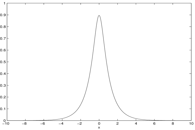
FIG. 1.: Soliton shape $r(x)$ with parameters $\mu=-1$, $\lambda=1$.

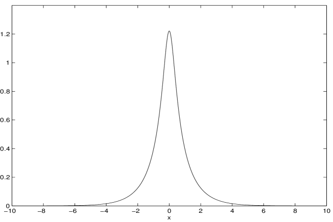
FIG. 2.: Soliton shape $r(x)$ with parameters $\mu=1$, $\lambda=1$.

For $\lambda=0$ and $\mu=1$ the iteration scheme gave the soliton dependence (Fig. 3), which is in agreement with the analytical result (V.13,V.14) at very high accuracy (for example, the factor $M$ at the stationary solution, presented in the paper, was equal to 1 within an error less than $10^{-5}$). The time step $\Delta\tau$ was equal to $0.00018$. All derivatives in the equations, as well as the action of the integral operator $\widehat{k}$, were calculated by means of the standard FFT program. The initial conditions for the iteration procedure (V.21) were taken in the form of solitons (V.9) with $\gamma=0$, which provide exponential decay while approaching the ends of the numerical interval on $x$. We chose a symmetric numerical domain $[-a,a]$, with $a=10$ for all runs except the case $\lambda=0$ where we took $a=50.$ The soliton shape in this particular case is presented in Fig. 3.

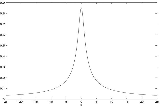
FIG. 3.: Soliton shape $r(x)$ with parameters $\mu=1$, $\lambda=0$.

Fig. 4 shows the dependence of $N$ on the soliton parameter $\lambda$. It is seen that the lower soliton branch and the upper soliton branch converge at large $\lambda$. Between the upper and the lower curves we have a straight line corresponding to the critical solitons with $N=N_{cr}$.

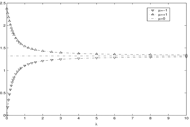
FIG. 4.: Dependence of $N$ on $\lambda$ for $\mu=\pm 1,0$

The same separation takes place for soliton amplitudes (Fig. 5). At the point $\lambda=0$ solitons undergo bifurcations.

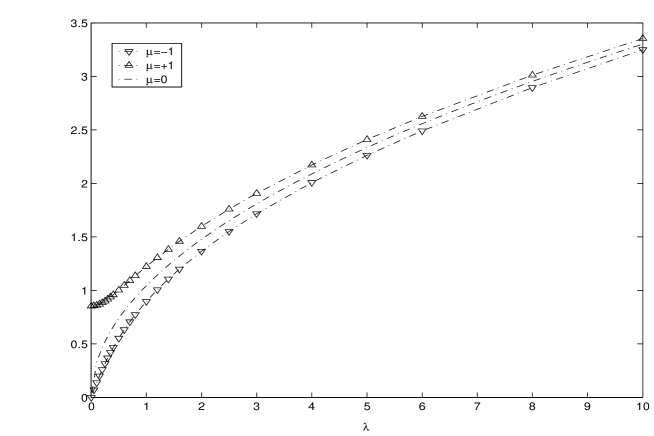
FIG. 5.: Dependence of soliton amplitude on $\lambda$

For negative $\mu$ we have a supercritical soliton bifurcation, while a subcritical occurs when $\mu>0$, with the soliton amplitude jump given by (V.14).

VI Stability of solitons

In this section we study the stability of the solitons that we analyzed in the previous section. In order to do that, we use the method based on Lyapunov’s theorem. Applying this theorem to the present Hamiltonian system means the following: a soliton considered as a stationary point of the Hamiltonian $\overline{H}$ for a fixed number of waves $N$ is stable if it realizes a minimum (or maximum) of the Hamiltonian. If a stationary point represents a saddle point then the corresponding soliton is expected to be unstable. The latter is only an indication that solitons are unstable. For instance, the classical counterexample is the Hamiltonian $H=p_{1}^{2}/2+q_{1}^{2}/2-p_{2}^{2}/2-q_{2}^{2}/2$ for a system with two degrees of freedom where the saddle point $p=q=0$ is stable.

In fact this type of indication is already available if one looks at the scaling (V.19,V.20) for which

$\displaystyle\overline{H}\left(a\right)=\left(\frac{1}{a}-\frac{1}{2a^{2}}\right)\frac{\mu}{2}\int r_{s}^{4}\,dx,$

where $r_{s}$ is the solitary wave solution. Hence, it is seen that for negative $\mu$ the function $\overline{H}\left(a\right)$ is bounded from below and its minimum, $\overline{H}_{s}<0,$ corresponds to the soliton. On the contrary, for $\mu>0$, this function has a maximum equal to $\overline{H}_{s}>0$, which is unbounded from below as $a\to 0$. Moreover, in the latter case, it is possible to see that the stationary point corresponding to the soliton solution is a saddle point. It follows immediately if, in addition to the scaling transformation, one considers the gauge transformation $\psi_{s}\rightarrow\psi_{s}e^{i\chi}$ under which

$\displaystyle\overline{H}\to\overline{H}_{s}+\int r^{2}\left(\chi_{x}\right)^{2}dx.$

For $\mu<0$, however, this transformation shows that the soliton solution remains the minimum point. We reach the same conclusion if we apply the Vakhitov-Kolokolov criterion [35] to the soliton solutions. The criterion states that, if

$\displaystyle\frac{\partial N_{s}}{\partial\lambda^{2}}<0,$

then solitons are unstable and they are stable in the opposite case. This criterion has a simple physical interpretation. The quantity $-\lambda^{2}$ is related to the energy of the soliton as a bound state. If by adding one particle (i.e. increasing $N$) this level shifts towards the continuous spectrum, then obviously such bound state will be unstable. As we saw in the previous section the derivative $\partial N_{s}/\partial\lambda^{2}$ is negative for $\mu>0$ and becomes positive when $\mu<0$ . We would like to emphasize that the Vakhitov-Kolokolov criterion was derived for the classical NLS equation and, strictly speaking, cannot be applied to our system. Thus, we have again indications that support stability of the lower soliton branch and, respectively, instability for the upper branch. Note that this stability indication is consistent with that for the cubic NLS solitons (V.8) which, as is well-known, are stable (see, e.g. [33]).

Now we show that the lower soliton branch ($\mu<0$) is stable: solitons from this branch indeed realize a minimum of the Hamiltonian $\overline{H}$ for a fixed number of waves $N$. The dimensionless Hamiltonian $\overline{H}$ written in terms of amplitude and phase reads

$$\overline{H}=\int\left[r_{x}{}^{2}+\frac{\mu}{2}r^{4}-\frac{\gamma}{2}r^{2}\widehat{k}r^{2}-\frac{1}{3}r^{6}+r^{2}\left(\varphi_{x}+\beta r^{2}\right)^{2}\right]dx.$$ (VI.1)

The last term here is positive definite and vanishes exactly on the stationary solitons. Thus, we now should prove that the minimum of $\overline{H}$ is reached on the soliton obtained as solution of Eq. (V.7).

Consider the integral

$\displaystyle I=\int\left[\frac{\gamma}{2}r^{2}\widehat{k}r^{2}+\frac{1}{3}r^{6}\right]dx$

and get its estimate through the integrals $\int r_{x}{}^{2}dx$ and $N$. As was shown in [10], we have the following estimate in the absence of nonlocal terms:

$\displaystyle\int r^{6}dx\leq\left(\frac{N}{N_{1}}\right)^{2}\int r_{x}{}^{2}\,dx,$

where $N_{1}=\int\psi_{0}{}^{2}dx$ and $\psi_{0}$ is the soliton solution for the quintic (critical) NLS equation,

$\displaystyle-\psi_{0}+\psi_{0xx}+3\psi_{0}^{5}=0.$

This solution can be easily found and gives $N_{1}=\pi/2$.

For the integral $I_{k}=\int r^{2}\widehat{k}r^{2}dx$, we can write the following set of inequalities:

$$\int r^{2}\widehat{k}r^{2}dx \leq \max_{x}\left(r^{2}\right)\int r\widehat{k}r\,dx\leq\int_{-\infty}^{x_{\max}}\left(r^{2}\right)_{x}\,dx\left(\int r^{2}dx\right)^{1/2}\left(\int r\widehat{k}^{2}r\,dx\right)^{1/2}$$

$$\leq C_{2}N\int r_{x}{}^{2}\,dx.$$

This inequality can be made sharper. To do that, consider the functional

$\displaystyle F\left\{r\right\}=\frac{\int r^{2}\widehat{k}r^{2}dx}{\int r^{2}dx\cdot\int r_{x}{}^{2}dx}.$

Its minimum value will give the best constant $C_{2}$. To find it one needs to determine a minimizer among all stationary points of the functional $F\left\{r\right\}$ . The stationary points of $F\left\{r\right\}$ are defined from the solutions of the equation

$\displaystyle 2r_{0}\widehat{k}r_{0}^{2}-r_{0}+r_{0xx}=0.$

The minimizer for $F\left\{r\right\}$ is given by the ground soliton solution of this equation. It is a symmetric function without nodes. Hence the best constant

$\displaystyle C_{2,\mathrm{best}}=\frac{1}{N_{2}},\quad N_{2}=\int r_{0}^{2}dx\approx 1.39035.$

Thus,

$$I\leq\left(\frac{\gamma}{2}\frac{N}{N_{2}}+\frac{N^{2}}{3N_{1}^{2}}\right)\int r_{x}{}^{2}dx.$$ (VI.2)

This inequality allows to find the criterion for the Hamiltonian to be bounded from below. Substituting (VI.2) into (VI.1) for $\mu<0$ yields

$$\overline{H}\geq\left[1-\left(\frac{\gamma}{2}\frac{N}{N_{2}}+\frac{N^{2}}{3N_{1}^{2}}\right)\right]\int r_{x}{}^{2}dx-\frac{1}{2}\int r^{4}\,dx.$$ (VI.3)

Hence it is seen that the Hamiltonian is bounded from below if

$\displaystyle\frac{\gamma}{2}\frac{N}{N_{2}}+\frac{N^{2}}{3N_{1}^{2}}\leq 1,$

or

$$N\leq N_{3}=\sqrt{\frac{9}{16}\gamma^{2}\frac{N_{1}^{4}}{N_{2}^{2}}+3N_{1}^{2}}-\frac{3}{4}\gamma\frac{N_{1}^{2}}{N_{2}}.$$ (VI.4)

The final step in proving the Hamiltonian boundedness is based on the estimate for the integral $\int r^{4}dx$. According to [15]

$\displaystyle\int r^{4}dx\leq\frac{1}{\sqrt{3}}N^{3/2}\left(\int r_{x}{}^{2}dx\right)^{1/2}.$

Substitution of this inequality into the estimate (VI.3) results in the desired bound for $\overline{H}$:

$\displaystyle\overline{H}\geq-\frac{N^{3}}{4\sqrt{3}}\left[1-\left(\frac{\gamma}{2}\frac{N}{N_{2}}+\frac{N^{2}}{3N_{1}^{2}}\right)\right].$

It turns out that the numerical value of $N_{3}=1.3224$ is almost the same as the critical number $N_{cr}=1.3225$, defined by solitons with $\mu=0$. Thus, solitons from the lower branch which satisfy the criterion (VI.4) are stable not only with respect to small perturbations but also against finite ones. Concerning the solitons from the upper branch, they are all unstable with respect to finite disturbances.

In summary, we would like to emphasize once more the difference between $N_{3}$ and $N_{cr}$ although the derivative $\partial N_{s}/\partial\lambda^{2}$ is positive for the whole lower soliton branch and according to the Vakhitov-Kolokolov criterion this branch is expected to be stable. Up to now it is an open question but we think that it is so and $N_{3}$ and $N_{cr}$ should coincide.

VII Concluding remarks

Thus, we have analyzed the behavior of solitons near the critical density ratio $\rho=\rho_{cr}$. Above $\rho_{cr}$ solitons undergo a subcritical bifurcation with the amplitude jump proportional to $\sqrt{\rho-\rho_{cr}}$. Therefore our theory based on the Hamiltonian expansion works when this jump is small, i.e. in a small vicinity of $\rho=\rho_{cr}$. In order to describe solitons a generalized NLS equation is derived based on the Hamiltonian average over fast oscillations with the carrying frequency corresponding to the critical soliton velocity $V=V_{cr}.$ The generalized NLS equation contains three kinds of nonlinear terms. The first one is nothing else than the nonlinear frequency shift taking into account six-wave nonlinear interactions. This is the local term. Another nonlinearity is responsible for steepening the envelope solitons (this is the so-called Lifshitz term [9]). And finally we have found the nonlocal contribution familiar to that calculated by Dysthe for gravity waves. This Dysthe term is focusing as well as the six-wave nonlinear interaction term. Within the generalized NLS equation we analyzed the stability of solitons. In particular, we have found a region of wave intensity, $N\leq N_{3}$, where solitons are stable. Their stability is based on the boundedness of the Hamiltonian from below. For solitons above $\rho_{cr}$ we have shown their possible instability, at least, instability with respect to finite perturbations. An interesting problem is the nonlinear stage of this instability, whether it can lead to the collapse of solitons. The latter question is important not only from the point of view of interfacial waves but also because there exists some similarity between the generalized NLS equation derived in this paper and those describing the behavior of short optical pulses in fibers from the femtosecond range of pulse durations.

A Six-wave coupling coefficient

As pointed out in Section III, the calculation of the nonlinear coupling coefficients $\beta$, $\gamma$ and of the six-wave coefficient $C$ can be performed independently for each coefficient. Therefore for the coefficient $C$ this problem reduces to the calculation of the nonlinear frequency shift for the main harmonic with $k=k_{0}$ and $\omega_{0}\equiv\omega(k_{0})$ when the first contribution to the nonlinear frequency shift proportional to $|\psi|^{2}$ is equal to zero. Second, in such a case, it is enough to consider its limit of a monochromatic wave, instead of a quasi-monochromatic wave. This means that one needs to develop the perturbation theory assuming that

$$a_{k}=\sqrt{2\pi}\sum_{n}C_{n}(t)e^{-in\omega_{0}t}\delta(k-nk_{0}),$$ (A.1)

where the leading order corresponds to the main harmonic $n=1$ and amplitudes of all other (combined) harmonics are supposed to be small in comparison with the first harmonic amplitude.

After this remark we introduce the small parameter $\epsilon$ so that

$$C_{1}=\epsilon\psi(T),$$ (A.2)

where $T=\epsilon^{4}t$ is a slow time and $\psi(T)$ is the envelope of the main harmonic. Hence it is easy to see that all needed combined harmonics $C_{n}$ become functions of the slow time $T$ and take in their expansion powers of the parameter $\epsilon$:

$$C_{0}=C_{0}^{*}=\epsilon^{2}\psi_{0}+\epsilon^{4}\psi_{01},\quad C_{\pm 2}=\epsilon^{2}\psi_{\pm 2}+\epsilon^{4}\psi_{\pm 21},\quad C_{-1}=\epsilon^{3}\psi_{-1},\quad C_{\pm 3}=\epsilon^{3}\psi_{\pm 3}.$$ (A.3)

Note that in this case nonlinear interactions with the zeroth harmonic do not give any contribution because the corresponding matrix elements vanish by the same law as for three-wave interaction.

The equations of motion for amplitudes $C_{n}$ follow from the general equation (II.9) for normal amplitude $a_{k}$:

$$\epsilon^{4}\frac{\partial C_{n}}{\partial T}+i\left[\omega(nk_{0})-n\omega_{0}\right]C_{n}=-i\frac{\partial\overline{H}_{\mathrm{int}}}{\partial C_{n}^{*}}.$$ (A.4)

Here $\overline{H}_{\mathrm{int}}$ is mean value of the interaction Hamiltonian after substitution expressions (A.1) into (III.1) and average. $\overline{H}_{\mathrm{int}}$ contains 19 matrix coefficients needed to determine the constant $C$ :

$$\ U_{11-2},\vskip 3.0pt plus 1.0pt minus 1.0pt\ U_{12-3},\vskip 3.0pt plus 1.0pt minus 1.0pt\ V_{1|-12},\vskip 3.0pt plus 1.0pt minus 1.0pt\ V_{1|-23},\vskip 3.0pt plus 1.0pt minus 1.0pt\ V_{-1|1-2},\vskip 3.0pt plus 1.0pt minus 1.0pt\ V_{2|11},\vskip 3.0pt plus 1.0pt minus 1.0pt\ V_{3|12},\vskip 3.0pt plus 1.0pt minus 1.0pt\ V_{-2|1-3},\vskip 3.0pt plus 1.0pt minus 1.0pt\ T_{11|11},\vskip 3.0pt plus 1.0pt minus 1.0pt\ T_{11|20},$$

$$T_{12|12},\vskip 3.0pt plus 1.0pt minus 1.0pt\ T_{1-2|1-2},\vskip 3.0pt plus 1.0pt minus 1.0pt\ T_{1|-111}^{(1,3)},\vskip 3.0pt plus 1.0pt minus 1.0pt\ T_{1|2-21}^{(1,3)},\vskip 3.0pt plus 1.0pt minus 1.0pt\ T_{3|111}^{(1,3)},\vskip 3.0pt plus 1.0pt minus 1.0pt\ T_{-3111}^{(0,4)},\vskip 3.0pt plus 1.0pt minus 1.0pt\ T_{1|-2111}^{(1,4)},\vskip 3.0pt plus 1.0pt minus 1.0pt\ T_{12|111}^{(2,3)},\vskip 3.0pt plus 1.0pt minus 1.0pt\ T_{111|111}^{(3,3)},$$

where $\pm 1\equiv\pm k_{0}$, $\pm 2\equiv\pm 2k_{0}$, and so on. These 19 coefficients are calculated in accordance with the rules explained in the third section.

As is seen from the equation of motion (A.4) the time derivative of $C_{n}$ is small compared with the second term $i\left[\omega(nk_{0})-n\omega_{0}\right]C_{n}$, except the main harmonic where this term vanishes. In its turn, the equation for $C_{1}$ contains terms proportional to $\epsilon^{3}$ and $\epsilon^{5}$. The terms of the third order ( $\sim$ $\epsilon^{3}$) are nothing more than the relation (IV.8) serving for definition of the critical Atwood number:

$\displaystyle T_{11|11}+\frac{2V_{2|11}^{2}}{2\omega_{1}-\omega_{2}}-\frac{2U_{11-2}^{2}}{2\omega_{1}+\omega_{2}}=0.$

The equation of motion for $\psi$ appears in the fifth order of $\epsilon$:

$$i\frac{\partial\psi}{\partial T} = 2U_{11-2}\psi^{*}\psi_{-21}^{*}+2U_{12-3}\psi_{2}^{*}\psi_{-3}^{*}+2V_{1|-12}\psi_{-1}\psi_{2}+2V_{1|-23}\psi_{-2}\psi_{3}$$

$$\ +2V_{-1|1-2}\psi_{-1}\psi_{-2}^{*}+2V_{2|11}\psi_{21}\psi^{*}\ +2V_{3|12}\psi_{3}\psi_{2}^{*}+2V_{-2|1-3}\psi_{-2}\psi_{-3}^{*}$$

$$\ +4T_{11|20}^{(2,2)}\psi^{*}\psi_{2}\psi_{0}+4T_{12|12}^{(2,2)}\psi_{2}^{*}\psi_{2}\psi+4T_{1-2|1-2}^{(2,2)}\psi_{-2}^{*}\psi_{-2}\psi+3T_{1|-111}^{(1,3)}\psi_{-1}\psi\psi$$

$$\ +6T_{1|2-21}^{(1,3)}\psi_{2}\psi_{-2}\psi+6T_{11-1|1}^{(3,1)}\psi\psi^{*}\psi_{-1}^{*}+6T_{12-2|1}^{(3,1)}\psi\psi_{2}^{*}\psi_{-2}^{*}+3T_{3|111}^{(3,1)}\psi_{3}\psi^{*}\psi^{*}$$

$$\ \ \ \ +12T_{-3111}^{(0,4)}\psi_{-3}^{*}\psi^{*}\psi^{*}+4T_{1|-2111}^{(1,4)}\psi_{-2}\psi\psi\psi+12T_{-2111|1}^{(4,1)}\psi\psi^{*}\psi^{*}\psi_{-2}^{*}\ \$$

$$\ +2T_{12|111}^{(2,3)}\psi_{2}^{*}\psi\psi\psi+6T_{111|21}^{(3,2)}\psi_{2}\psi\psi^{*}\psi^{*}\ \ +3T_{111|111}^{(3,3)}|\psi|^{4}\psi$$

where all matrix elements are defined without factors of $\left(\sqrt{2\pi}\right)^{2-n-m}$ as they had according to the definition of Section III (compare with (III.26), (III.28), III.30)).

Here the amplitudes $\psi_{0},\psi_{01},\psi_{\pm 2},\psi_{\pm 21},\psi_{-1},\psi_{\pm 3}\$ are found with the help of equations (A.4). This is a pure algebraic procedure which we performed with the help of computer. As the result of substitution of $\psi_{0},\psi_{01},\psi_{\pm 2},\psi_{\pm 21},\psi_{-1},\psi_{\pm 3}$ into the above equation we arrive at the equation:

$\displaystyle i\frac{\partial\psi}{\partial T}=3\widetilde{T}_{111|111}^{(3,3)}|\psi|^{4}\psi,$

where the six-wave coupling coefficient $C$ is positive:

$\displaystyle C=-\widetilde{T}_{111|111}^{(3,3)}=\frac{Mk_{0}^{6}}{3\omega_{0}},\vskip 3.0pt plus 1.0pt minus 1.0pt\ M=\frac{289(21+8\sqrt{5})}{16384}\approx 0.685961.$

The corresponding nonlinear term is focusing.

REFERENCES

[1] M. S. Longuet-Higgins, Capillary-gravity waves of
solitary type on deep water, J. Fluid Mech. 200, 451-470 (1989).
[2] G. Iooss and K. Kirchgässner, Bifurcation d’ondes
solitaires en présence d’une faible tension superficielle, C. R. Acad.
Sci. Paris, Série I 311, 265-268 (1990).
[3] J.-M. Vanden-Broeck and F. Dias, Gravity-capillary
solitary waves in water of infinite depth and related free-surface flows,
J. Fluid Mech. 240, 549-557 (1992).
[4] F. Dias and G. Iooss, Capillary-gravity solitary
waves with damped oscillations, Physica D 65, 399-423 (1993).
[5] M. S. Longuet-Higgins, Capillary-gravity waves of
solitary type and envelope solitons on deep water, J. Fluid Mech. 252, 703-711 (1993).
[6] T. R. Akylas, Envelope solitons with stationary
crests, Phys. Fluids 5, 789-791 (1993).
[7] F. Dias and G. Iooss, Capillary-gravity interfacial
waves in deep water, Eur. J. Mech. B/Fluids 15, 367-390 (1996).
[8] P.-O. Rusas and J. Grue, Solitary waves and
conjugate flows in a three-layer fluid, Eur. J. Mech. B/Fluids 21,
185-206 (2002).
[9] L. D. Landau and E. M. Lifshitz, Statistical Physics,
Part 1 (Pergamon Press, New York) [Russian original: Nauka, Moscow, 1995,
p. 521].
[10] E. A. Kuznetsov, Hard soliton excitation: stability
investigation, ZhETF 116, 299-317 (1999) [JETP 89,
163-172 (1999)].
[11] S. M. Sun, Some analytical properties of
capillary-gravity waves in two-fluid flows of infinite depth, Proc. R. Soc.
Lond. A 453, 1153-1175 (1997).
[12] K. B. Dysthe, Note on a modification to the
nonlinear Schrödinger equation for application to deep water waves, Proc.
R. Soc. Lond. A 369, 105-114 (1979).
[13] M. J. Ablowitz, J. Hammack, D. Henderson and C. M.
Schober, Modulated periodic Stokes waves in deep water, Phys. Rev.
Lett. 84, 887-890 (2000); Long-time dynamics of the
modulational instability of deep water waves, Physica D 152-153,
416-433 (2001).
[14] V. E. Zakharov and E. A. Kuznetsov, Hamiltonian
formalism for nonlinear waves, Usp. Fiz. Nauk 167, 1137-1168
(1997) [Physics-Uspekhi 40, 1087-1116 (1997)].
[15] V. E. Zakharov and E. A. Kuznetsov, Optical solitons
and quasisolitons, Zh. Éksp. Teor. Fiz. 113, 1892 (1998) [JETP
86, 1035-1046 (1998)].
[16] Yu. A. Sinitsyn and V. M. Kontorovich, In: Studies of
Turbulent Structure of Ocean, Ed. by Ozmidov, Izd. MGI, Sevastopol’ (1975)
(first Symposium “Issledovanie melkomaschtabnoi okeanicheskoi
turbulentnosti”, Kaliningrad, 1974); V. M. Kontorovich, A possible
role of internal waves in occurence of small-scale turbulence in stratified
ocean. Izv. Vuzov, Radiofizika 19, 872-879 (1976).
[17] E. A. Kuznetsov and M. D. Spector, Existence of
hexagon relief on the surface of the liquid dielectrics in an external
electric field, Zh. Éksp. Teor. Fiz. 71, 262 (1976) [Sov. Phys.
JETP 44, 136 (1976)].
[18] E. A. Kuznetsov, M. D. Spector and V. E. Zakharov,
Surface singularities of ideal fluid, Phys.Lett. 182A,
387-393, (1993).
[19] F. Dias and T. Bridges, Geometric aspects of
spatially periodic interfacial waves, Stud. Appl. Math. 93, 93-132
(1994).
[20] V. E. Zakharov, Stability of periodic waves of
finite amplitude on the surface of a deep fluid, Zh. Prikl. Mekh. Tekh.
Fiz. 9, 86-94 (1968) [J. Appl. Mech. Tech. Phys. 9,
190-194 (1968)]; V. E. Zakharov and N. N. Filonenko, The energy
spectrum for stochastic oscillations of a fluid surface, Doclady Akad. Nauk
SSSR 170, 1292-1295 (1966) [Sov. Phys. Docl. 11, 881-884
(1967)].
[21] T. B. Benjamin and T. J. Bridges, Reappraisal of the
Kelvin-Helmholtz problem. I. Hamiltonian structure, J. Fluid Mech. 333, 301-325 (1997).
[22] W. Craig and M. D. Groves, Normal forms for wave
motion in fluid interfaces, Wave Motion 31, 21-41 (2000).
[23] W. Craig, P. Guyenne, and H. Kalisch, Hamiltonian
long wave expansions for free surfaces and interfaces, Comm. Pure Appl.
Math. 58, 1587-1641 (2005).
[24] V.E. Zakharov, Kolmogorov spectra in weak turbulence
problems, in: Handbook of Plasma Physics, Vol. 2, Basic Plasma Physics,
eds. A.A. Galeev, R.N. Sudan (Elsevier, North-Holland, 1984), pp. 3-36.
[25] A. C. Newell, Solitons in Mathematics and Physics
(SIAM, Philadelphia, 1985).
[26] F. Dias and E. A. Kuznetsov, On the nonlinear
stability of solitary waves for the fifth-order Korteweg-de Vries equation,
Phys. Letters A 263, 98-104 (1999).
[27] O. Laget and F. Dias, Numerical computation of
capillary-gravity interfacial solitary waves, J. Fluid Mech. 349,
221-251 (1997).
[28] T. J. Bridges, P. Christodoulides and F. Dias, Spatial bifurcations of interfacial waves when the phase and group
velocities are nearly equal, J. Fluid Mech. 285, 121-158 (1995).
[29] A. I. Dyachenko, A. O. Korotkevich, and V. E.
Zakharov, Weak turbulent Kolmogorov spectrum for surface gravity
waves, Phys. Rev. Lett. 92, 134501 (2004).
[30] V. E. Zakharov, V. S. L’vov, The statistical
description of the nonlinear wave fields, Izv. Vuzov, Radiofizika 18, 1470-1487 (1975).
[31] G. Iooss, Existence d’orbites homoclines à un
équilibre elliptique, pour un système réversible, C. R. Acad. Sci.
Paris 324, 993-997 (1997).
[32] E. A. Kuznetsov and S. K. Turitsyn, Talanov
Transformations for Selffocusing Problems and Instability of Waveguides.
Phys.Lett. 112A, 273 (1985).
[33] E. A. Kuznetsov, A. M. Rubenchik, and V. E. Zakharov, Soliton Stability in Plasmas and Fluids, Phys. Rep. 142, 103
(1986).
[34] V. I. Petviashvili, On the Equation for
Unusual Soliton, Fizika Plasmy, 2, 469-472 (1976) [Sov. J. Plasma
Phys., 2, 247-250 (1976)]; Non-one-dimensional Solitons,
in: ”Nonlinear waves”, ed. A.V. Gaponov-Grekhov, Moscow, Nauka, 1979, pp.
5-21.
[35] N. G. Vakhitov, A. A. Kolokolov, Stationary solutions
of the wave equation in media with saturated nonlinearity, Izv. VUZ
Radiofizika 16, 1020-1028 (1973) [Radiophys. Quant. Electron.
16, 783 (1973)] .