Abstract

The Bergman–Milton bounds provide limits on the effective permittivity of a composite material comprising two isotropic dielectric materials. These provide tight bounds for composites arising from many conventional materials. We reconsider the Bergman–Milton bounds in light of the recent emergence of metamaterials, in which unconventional parameter ranges for relative permittivities are encountered. Specifically, it is demonstrated that: (a) for nondissipative materials the bounds may be unlimited if the constituent materials have relative permittivities of opposite signs; (b) for weakly dissipative materials characterized by relative permittivities with real parts of opposite signs, the bounds may be exceedingly large.

Keywords: Bergman–Milton bounds; Maxwell Garnett estimates; Hashin–Shtrikman bounds; metamaterials

1 Introduction

Increasingly, new materials which exhibit novel and potentially useful electromagnetic responses are being developed [1, 2]. At the forefront of this rapidly expanding field lie metamaterials [3]. These are artificial composite materials which exhibit properties that are either not exhibited by their constituents at all, or not exhibited to the same extent by their constituents. With the emergence of these new materials — which may exhibit radically different properties to those encountered traditionally in electromagnetics/optics — some re–evaluation of established theories is necessary. A prime example is provided by the recent development of metamaterials which support planewave propagation with negative phase velocity [4]. The experimental demonstration of negative refraction in 2000 prompted an explosion of interest in issues pertaining to negative phase velocity and negative refraction [5, 6].

The process of homogenization, whereby two (or more) homogeneous constituent materials are blended together to produce a composite material which is effectively homogeneous within the long–wavelength regime, is an important vehicle in the conceptualization of metamaterials [7]. The estimation of the effective constitutive parameters of homogenized composite materials (HCMs) is a well–established process [8], aspects of which have been revisited recently in light of the development of exotic materials that exhibit properties such as negative phase velocity. For example, it was demonstrated that two widely used homogenized formalisms, namely the Maxwell Garnett and Bruggeman formalisms, do not provide useful estimates of the HCM permittivity within certain parameter regimes [9]. The Maxwell Garnett estimates coincide with the well–known Hashin–Shtrikman bounds [10] on the HCM permittivity. While the former are commonly implemented for both dissipative and nondissipative HCMs, the later were derived for nondissipative HCMs.

In view of the limitations of the Maxwell Garnett and Bruggeman formalisms within certain parameter regimes, we explore in this communication the implementation of the Bergman–Milton bounds [11, 12, 13] for these parameter regimes. To be specific, we consider the homogenization of two isotropic dielectric constituent materials with relative permittivities $\epsilon_{a}$ and $\epsilon_{b}$. We explore the regime in which the parameter

$$\delta=\frac{\mbox{Re}\left(\epsilon_{a}\right)}{\mbox{Re}\left(\epsilon_{b}\right)}\,,\qquad\qquad(\epsilon_{a},\epsilon_{b}\in\mathbb{C})\,,$$ (1)

is negative–valued, as this is where the Maxwell Garnett and Bruggeman estimates are not useful [9]. Notice that the definition (1) caters to the possibility that only one of $\epsilon_{a}$ or $\epsilon_{b}\in\mathbb{R}$, as might arise for a metal–in–insulator HCM, for example. In fact, the $\delta<0$ regime which occurs for metal–in–insulator HCMs [14, 15] is highly pertinent to the homogenization of HCMs which support planewave propagation with negative phase velocity.

Let us note that, although the $\delta<0$ regime has been discussed in the past in the context of the Bergman–Milton bounds [12, 15, 16], the discussion on the inadequacy of those bounds has been brief. Amplification is needed because of the possibility of fabricating negatively refracting composite materials [17, 18], for example.

2 Bergman–Milton bounds

Two bounds on the effective relative permittivity $\epsilon_{e}$ of the chosen composite material were established by Bergman [11, 19, 20, 21] and Milton [12, 22]. We write these as $\mathsf{BM}_{\alpha}$ and $\mathsf{BM}_{\beta}$. In terms of a real–valued parameter $\gamma$, these are given by (see eqn. (24) in [12])

$$\mathsf{BM}_{\alpha}(\gamma)=f_{a}\epsilon_{a}+f_{b}\epsilon_{b}-\frac{f_{a}f_{b}(\epsilon_{b}-\epsilon_{a})^{2}}{3\left[\gamma\epsilon_{a}+\left(1-\gamma\right)\epsilon_{b}\right]}\,,\qquad\qquad(\epsilon_{a},\epsilon_{b}\in\mathbb{C})\,,$$ (2)

and

$$\mathsf{BM}_{\beta}(\gamma)=\left\{\frac{f_{a}}{\epsilon_{a}}+\frac{f_{b}}{\epsilon_{b}}-\frac{2f_{a}f_{b}\left(\epsilon_{a}-\epsilon_{b}\right)^{2}}{3\,\epsilon_{a}\epsilon_{b}\left[\epsilon_{b}\gamma+\epsilon_{a}\left(1-\gamma\right)\right]}\right\}^{-1},\qquad\qquad(\epsilon_{a},\epsilon_{b}\in\mathbb{C})\,,$$ (3)

where $f_{a,b}$ denotes the volume fraction of the constituent material with relative permittivity $\epsilon_{a,b}$, and $f_{a}+f_{b}=1$. For the bound $\mathsf{BM}_{\alpha}$ the parameter $\gamma$ takes the values $\left(1-f_{a}\right)/3\leq\gamma\leq 1-f_{a}/3$, whereas for the bound $\mathsf{BM}_{\beta}$ the parameter $\gamma$ takes the values $2\left(1-f_{a}\right)/3\leq\gamma\leq 1-2f_{a}/3$.

The Bergman–Milton bounds (2) and (3) are related to the two Maxwell Garnett estimates of the HCM relative permittivity [8, 14]

$$\mathsf{MG}_{\alpha}=\epsilon_{b}+\frac{3f_{a}\epsilon_{b}(\epsilon_{a}-\epsilon_{b})}{\epsilon_{a}+2\epsilon_{b}-f_{a}(\epsilon_{a}-\epsilon_{b})},\qquad\qquad(\epsilon_{a},\epsilon_{b}\in\mathbb{C})\,,$$ (4)

$$\mathsf{MG}_{\beta}=\epsilon_{a}+\frac{3f_{b}\epsilon_{a}(\epsilon_{b}-\epsilon_{a})}{\epsilon_{b}+2\epsilon_{a}-f_{b}(\epsilon_{b}-\epsilon_{a})},\qquad\qquad(\epsilon_{a},\epsilon_{b}\in\mathbb{C})\,.$$ (5)

The Maxwell Garnett estimates represent the extension of the Hashin–Shtrikman bounds [10] into the complex–valued permittivity regime. For nondissipative HCMs, the Maxwell Garnett estimates coincide with the Bergman–Milton bounds when the parameter $\gamma$ attains its minimum and maximum values; i.e.,

$$\left.\begin{array}[]{lllll}\displaystyle{\mathsf{BM}_{\alpha}\left(\frac{1-f_{a}}{3}\right)}&=&\displaystyle{\mathsf{BM}_{\beta}\left(\frac{2-2f_{a}}{3}\right)}&=&\mathsf{MG}_{\alpha}\\ &&&&\\ \displaystyle{\mathsf{BM}_{\alpha}\left(1-\frac{f_{a}}{3}\right)}&=&\displaystyle{\mathsf{BM}_{\beta}\left(1-\frac{2f_{a}}{3}\right)}&=&\mathsf{MG}_{\beta}\end{array}\right\}\,.$$ (6)

In view of our particular interest in homogenization scenarios for which $\delta<0$, we note that

$$\left|\mathsf{BM}_{\alpha}\left(\frac{1-f_{a}}{3}\right)\right|=\left|\mathsf{BM}_{\beta}\left(\frac{2-2f_{a}}{3}\right)\right|=\left|\mathsf{MG}_{\alpha}\right|\rightarrow\infty\qquad\mbox{as}\qquad\delta\rightarrow\frac{f_{b}-3}{f_{b}}\,$$ (7)

and

$$\left|\mathsf{BM}_{\alpha}\left(1-\frac{f_{a}}{3}\right)\right|=\left|\mathsf{BM}_{\beta}\left(1-\frac{2f_{a}}{3}\right)\right|=\left|\mathsf{MG}_{\beta}\right|\rightarrow\infty\qquad\mbox{as}\qquad\delta\rightarrow\frac{f_{a}}{f_{a}-3}\,$$ (8)

for nondissipative mediums. Thus, there exist

• a volume fraction $f_{a}\in\left(0,1\right)$ at which $\mathsf{MG}_{\alpha}$ is unbounded for all values of $\delta<-2$, and

• a volume fraction $f_{a}\in\left(0,1\right)$ at which $\mathsf{MG}_{\beta}$ is unbounded for all values of $\delta\in\left(-1/2,0\right)$.

3 Numerical illustrations

Let us now numerically explore the Bergman–Milton bounds, along with the Maxwell Garnett estimates, for some illustrative examples of nondissipative and dissipative HCMs. The parameter $\delta$, defined in (1), is used to classify the two constituent materials of the chosen HCMs. We begin in §3.1 by considering nondissipative HCMs. While these do not represent realistic materials, they provide valuable insights into the limiting process in which weakly dissipative materials become nondissipative. Furthermore, they provide a useful yardstick in the evaluation of dissipative HCMs, which are considered in §3.2.

3.1 Nondissipative HCMs

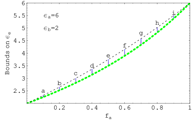
Figure 1: The $\mathsf{MG}_{\alpha}$ (thick dashed line) and $\mathsf{MG}_{\beta}$ (thin dashed line) estimates of $\epsilon_{e}$ plotted against $f_{a}$ for $\epsilon_{a}=6$, $\epsilon_{b}=2$. The vertical solid lines represent the variation of the Bergman–Milton bound $\mathsf{BM}_{\alpha}$ with $\gamma$ for $f_{a}\in\{0.1(a),0.2(b),0.3(c),0.4(d),0.5(e),0.6(f),0.7(g),0.8(h),0.9(i)\}$; and these coincide with the corresponding variation of $\mathsf{BM}_{\beta}$ with $\gamma$.

We begin with the most straightforward situation: nondissipative HCMs arising from constituent materials with $\delta>0$. In Figure 1, the Maxwell Garnett estimates $\mathsf{MG}_{\alpha}$ and $\mathsf{MG}_{\beta}$ (which in this case are identical to the Hashin–Shtrikman bounds) are plotted against $f_{a}\in(0,1)$ for $\epsilon_{a}=6$ and $\epsilon_{b}=2$. The Bergman–Milton bound $\mathsf{BM}_{\alpha}$ is given for $f_{a}\in\left\{0.1,0.2,0.3,0.4,0.5,0.6,0.7,0.8,0.9\right\}$. The corresponding plots of $\mathsf{BM}_{\beta}(\gamma)$ with $\gamma$ overlies that of $\mathsf{BM}_{\alpha}$. The Bergman–Milton bounds are entirely contained within the envelope constructed by the Maxwell Garnett estimates.

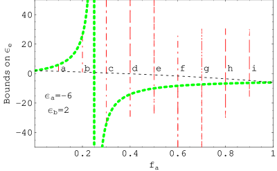
Figure 2: The $\mathsf{MG}_{\alpha}$ (thick dashed line) and $\mathsf{MG}_{\beta}$ (thin dashed line) estimates of $\epsilon_{e}$ plotted against $f_{a}$ for $\epsilon_{a}=-6$ and $\epsilon_{b}=2$. The Bergman–Milton bound $\mathsf{BM}_{\alpha}$ is plotted as the vertical broken lines for $f_{a}\in\{0.1(a),0.2(b),0.3(c),0.4(d),0.5(e),0.6(f),0.7(g),0.8(h),0.9(i)\}$.

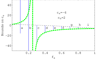
Figure 3: As Figure 2 but with $\mathsf{BM}_{\beta}$ (vertical solid lines) in place of $\mathsf{BM}_{\alpha}$.

Let us turn now to the nondissipative scenario wherein $\delta<0$. In Figure 2, the the Maxwell Garnett estimates $\mathsf{MG}_{\alpha}$ and $\mathsf{MG}_{\beta}$ are presented as functions of $f_{a}$ for $\epsilon_{a}=-6$ and $\epsilon_{b}=2$. The Bergman–Milton bound $\mathsf{BM}_{\alpha}$ is given for $f_{a}\in\left\{0.1,0.2,0.3,0.4,0.5,0.6,0.7,0.8,0.9\right\}$. The corresponding Bergman–Milton bound $\mathsf{BM}_{\beta}$ is plotted in Figure 3. In consonance with (6) and (7), we see that $\mathsf{MG}_{\alpha}$ becomes unbounded as $f_{a}\rightarrow 0.25$. It is clear that $\mathsf{MG}_{\beta}\leq\mathsf{BM}_{\alpha}\leq\mathsf{MG}_{\alpha}$ for $f_{a}<0.25$, whereas $\mathsf{MG}_{\alpha}\leq\mathsf{BM}_{\beta}\leq\mathsf{MG}_{\beta}$ for $f_{a}>0.25$. For $f_{a}>0.25$, the Bergman–Milton bound $\mathsf{BM}_{\alpha}$ lies outside both Maxwell Garnett estimates $\mathsf{MG}_{\alpha}$ and $\mathsf{MG}_{\beta}$, and similarly $\mathsf{BM}_{\beta}$ lies outside both Maxwell Garnett estimates $\mathsf{MG}_{\alpha}$ and $\mathsf{MG}_{\beta}$ for $f_{a}<0.25$, although the relations (6) still hold.

3.2 Dissipative HCMs

We turn to homogenization scenarios based on dissipative constituent materials; i.e., $\epsilon_{a,b}\in\mathbb{C}$. Let us begin with the $\delta>0$ scenario. In Figure 4, the homogenization of constituents characterized by the relative permittivities $\epsilon_{a}=6+0.3i$ and $\epsilon_{b}=2+0.2i$ is illustrated. In this figure, the Maxwell Garnett estimates on complex–valued $\epsilon_{e}$ are plotted as $f_{a}$ varies from $0$ to $1$. The Bergman–Milton bounds, which are graphed for $f_{a}\in\left\{0.1,0.2,0.3,0.4,0.5,0.6,0.7,0.8,0.9\right\}$, are fully contained within the Maxwell Garnett envelope. That is, we have $\mathsf{MG}_{\beta}\leq\mathsf{BM}_{\alpha,\beta}\leq\mathsf{MG}_{\alpha}$ for all values of $f_{a}$.

Now we consider dissipative constituent materials with $\delta<0$. In Figure 5, the homogenization of constituent materials given by $\epsilon_{a}=-6+3i$ and $\epsilon_{b}=2+2i$ is represented. The Maxwell Garnett estimates are plotted for $f_{a}\in(0,1)$, whereas the Bergman–Milton bounds are given for $f_{a}\in\left\{0.1,0.2,0.3,0.4,0.5,0.6,0.7,0.8,0.9\right\}$. As is the case in Figure 4, $\mathsf{BM}_{\beta}$ lies entirely within the envelope constructed by $\mathsf{MG}_{\alpha}$ and $\mathsf{MG}_{\beta}$. We see that $\mathsf{BM}_{\alpha}\geq\mathsf{MG}_{\beta}$ for all values of $f_{a}$; but, for mid–range values of $f_{a}$, $\mathsf{BM}_{\alpha}$ slightly exceeds $\mathsf{MG}_{\alpha}$ for certain values of the parameter $\gamma$.

As the degree of dissipation exhibited by the constituent materials is decreased, the extent to which $\mathsf{BM}_{\alpha}$ exceeds $\mathsf{MG}_{\alpha}$ is increased. This is illustrated in Figure 6 wherein the homogenization is repeated with $\epsilon_{a}=-6+i$ and $\epsilon_{b}=2+2i/3$. As in Figure 4, the Maxwell Garnett estimates are plotted for $f_{a}\in(0,1)$, while the Bergman–Milton bounds are given for $f_{a}\in\left\{0.1,0.2,0.3,0.4,0.5,0.6,0.7,0.8,0.9\right\}$. The Bergman–Milton bound $\mathsf{BM}_{\beta}$ lies within the Maxwell Garnett envelope for all values of $f_{a}$, but substantial parts of $\mathsf{BM}_{\alpha}$ lie well outside the envelope of the two Maxwell Garnett estimates.

The behaviour observed in Figures 5 and 6 is further exaggerated in Figure 7, where the homgenization of constituent materials with $\epsilon_{a}=-6+0.3i$ and $\epsilon_{b}=2+0.2i$ is represented. The Maxwell Garnett estimates are plotted for $f_{a}\in(0,1)$; for reasons of clarity, the Bergman–Milton bounds are plotted only for $f_{a}\in\left\{0.1,0.3,0.5\right\}$. The Maxwell Garnett estimates are exceedingly large and the Bergman–Milton bounds are larger still.

Finally, let us focus on the scenario referred to in the introduction, namely the homogenization of a conducting constituent material and a nonconducting constituent material, wherein $\delta<0$. Suppose we consider constituents characterized by the relative permittivities $\epsilon_{a}=-6+3i$ and $\epsilon_{b}=2$. In Figure 8 the Maxwell Garnett estimates are plotted for $f_{a}\in(0,1)$, whereas the Bergman–Milton bounds are given for $f_{a}\in\left\{0.1,0.2,0.3,0.4,0.5,0.6,0.7,0.8,0.9\right\}$. As we observed in Figure 6, the Maxwell Garnett envelope does not contain substantial parts of the Bergman–Milton bound $\mathsf{BM}_{\alpha}$, whereas the $\mathsf{BM}_{\beta}$ bound lies entirely within the envelope constructed from the two Maxwell Garnet estimates.

4 Discussion and conclusions

The Bergman–Milton bounds, as well as the Maxwell Garnett estimates, are valuable for estimating the effective constitutive parameters of HCMs in many commonly encountered circumstances. However, the advent of exotic new materials and metamaterials has led to the examination of such bounds within unconventional parameter regimes. It was recently demonstrated that the Bruggeman homogenization formalism and the Maxwell Garnett homogenization formalism do not provide useful estimates of the HCM permittivity when the relative permittivities of the constituent materials $\epsilon_{a}$ and $\epsilon_{b}$ are such that [9]

• $\mbox{Re}\left(\epsilon_{a}\right)$ and $\mbox{Re}\left(\epsilon_{b}\right)$ have opposite signs; and

• $|\mbox{Re}\left(\epsilon_{a,b}\right)|$ $\gg$ $|\mbox{Im}\left(\epsilon_{a,b}\right)|$.

Similarly, we have demonstrated in the preceding sections of this communication, that the Bergman–Milton bounds do not provide tight limits on the value of $\epsilon_{e}$ within the same parameter regime.

We note that if the real parts of $\epsilon_{a}$ and $\epsilon_{b}$ have opposite signs, but are of the same order of magnitude as their imaginary parts, then the Bergman–Milton bounds are indeed useful, and they then lie within the envelope constructed by the Maxwell Garnett estimates.

Acknowledgement: AL is grateful for many discussions with Bernhard Michel of Scientific Consulting, Rednitzhembach, Germany. The authors thank anonymous referees for their helpful remarks.

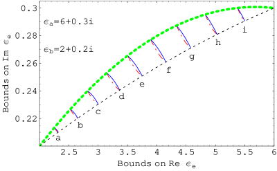
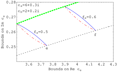
Figure 4: The $\mathsf{MG}_{\alpha}$ (thick dashed line) and $\mathsf{MG}_{\beta}$ (thin dashed line) estimates in relation to $\mbox{Re}\,\epsilon_{e}$ and $\mbox{Im}\,\epsilon_{e}$ as $f_{a}$ varies from $0$ to $1$, for $\epsilon_{a}=6+0.3i$, $\epsilon_{b}=2+0.2i$. The Bergman–Milton bounds $\mathsf{BM}_{\alpha}$ (thin broken dashed lines) and $\mathsf{BM}_{\beta}$ (thin solid lines) in the top diagram are plotted for $f_{a}\in\{0.1(a),0.2(b),0.3(c),0.4(d),0.5(e),0.6(f),0.7(g),0.8(h),0.9(i)\}$. The bottom diagram shows the Bergman–Milton bounds in greater detail but for $f_{a}=0.5(e)$ and $f_{a}=0.6(f)$.

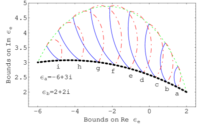
Figure 5: The $\mathsf{MG}_{\alpha}$ (thin dashed line) and $\mathsf{MG}_{\beta}$ (thick dashed line) estimates in relation to $\mbox{Re}\,\epsilon_{e}$ and $\mbox{Im}\,\epsilon_{e}$ as $f_{a}$ varies from $0$ to $1$, for $\epsilon_{a}=-6+3i$ and $\epsilon_{b}=2+2i$. The Bergman–Milton bounds $\mathsf{BM}_{\alpha}$ (thin broken dashed lines) and $\mathsf{BM}_{\beta}$ (thin solid lines) are plotted for $f_{a}\in\{0.1(a),0.2(b),0.3(c),0.4(d),0.5(e),0.6(f),0.7(g),0.8(h),0.9(i)\}$.

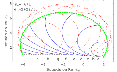
Figure 6: As Figure 4 but for $\epsilon_{a}=-6+i$, $\epsilon_{b}=2+2i/3$.

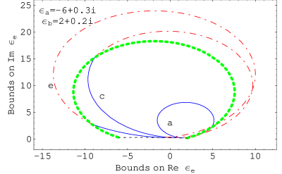
Figure 7: As Fig. 4 but for $\epsilon_{a}=-6+0.3i$ and $\epsilon_{b}=2+0.2i$. The Bergman–Milton bounds are plotted for $f_{a}\in\{0.1(a),0.3(c),0.5(e)\}$.

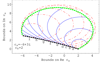
Figure 8: As Fig. 4 but for $\epsilon_{a}=-6+3i$ and $\epsilon_{b}=2$.

References

- [1] W.S. Weiglhofer, A. Lakhtakia (Eds.), Introduction to Complex Mediums for Optics and Electromagnetics, SPIE, Bellingham, WA, USA, 2003.
- [2] O.N. Singh, A. Lakhtakia (Eds.), Electromagnetic Fields in Unconventional Materials and Structures, Wiley, New York, NY, USA, 2000.
- [3] R.M. Walser, in: W.S. Weiglhofer, A. Lakhtakia (Eds.), Introduction to Complex Mediums for Optics and Electromagnetics, SPIE, Bellingham, WA, USA, 2003, pp. 295–316.
- [4] Focus on Negative Refraction, New J. Phys. 7 (2005). http://dx.doi.org/10.1088/1367-2630/7/1/E03
- [5] A.D. Boardman, N. King, L. Velasco, Electromagnetics 25 (2005) 365.
- [6] S.A. Ramakrishna, Rep. Prog. Phys. 68 449.
- [7] T.G. Mackay, Electromagnetics 25 (2005) 461.
- [8] A. Lakhtakia (Ed.), Selected Papers on Linear Optical Composite Materials, SPIE, Bellingham, WA, USA, 1996.
- [9] T.G. Mackay, A. Lakhtakia, Opt. Commun. 234 (2004) 35.
- [10] Z. Hashin, S. Shtrikman, J. Appl. Phys. 33 (1962) 3125.
- [11] D.J. Bergman, Phys. Rev. B. 23 (1981) 3058.
- [12] G.W. Milton, J. Appl. Phys. 52 (1981) 5286.
- [13] D.J. Bergman, Phys. Rev. Lett. 44 (1980) 1285.
- [14] D.E. Aspnes, Am. J. Phys. 50 (1982) 704. (Reproduced in [8]).
- [15] G.W. Milton, Appl. Phys. Lett. 37 (1980) 300.
- [16] G.W. Milton, Phys. Rev. Lett. 46 (1981) 542.
- [17] T.G. Mackay, A. Lakhtakia, Microw. Opt. Technol. Lett. 47 (2005) 313.
- [18] T.G. Mackay, A. Lakhtakia, Microw. Opt. Technol. Lett. 48 (2006) at press.
- [19] D.J. Bergman, Phys. Rep. 43 (1978) 378.
- [20] D.J. Bergman, Annals. Phys. 138 (1982) 78.
- [21] D.J. Bergman, SIAM J. Appl. Math. 53 (1993) 915.
- [22] G.W. Milton, The Theory of Composites, Cambridge University Press, Cambridge, UK, 2002.