Multistage Random Growing Small-World Networks with Power-law degree Distribution

Abstract

In this paper, a simply rule that generates scale-free networks with very large clustering coefficient and very small average distance is presented. These networks are called Multistage Random Growing Networks(MRGN) as the adding process of a new node to the network is composed of two stages. The analytic results of power-law exponent $\gamma=3$ and clustering coefficient $C=0.81$ are obtained, which agree with the simulation results approximately. In addition, the average distance of the networks increases logarithmical with the number of the network vertices is proved analytically. Since many real-life networks are both scale-free and small-world networks, MRGN may perform well in mimicking reality.

The past few years have witnessed a great devotion by physicists to understand and characterize the underlying mechanisms of complex networks including the Internet, the World Wide Web, the scientific collaboration networks and so onWS98 ; BA99 ; AB02 ; DM02 ; New ; XFWang01 . The results of many experiments and statistical analysis indicate that the networks in various fields have some common characteristics. They have a small average distance like random graphs, a large clustering coefficient and power-law degree distribution WS98 ; BA99 , which is called the small-world and scale-free characteristics. Recent works on the mathematics of networks have been driven largely by the empirical properties of real-life networksE1 ; E2 ; E3; E4 ; E5 ; E6 ; E7 ; E8 ; E9 and the studies on network dynamicsD1 ; D2 ; D3 ; D4 ; D5 ; D6 ; D7 ; D8 ; D9 ; D10 ; D11 ; D12 ; D13 ; D14 ; D15 , optimizationO1 ; O2 ; O3 ; O4 ; O5 ; O6 and evolutionary M1 ; M2 ; M3 ; M4 ; M5 ; M6 ; M7 ; M8 ; M9 ; M10 ; M11 ; M12 ; M13 . The first successful attempt to generate networks with high clustering coefficients and small average distance is that of Watts and Strogatz (WS model) WS98 . Another significant model is proposed by Barabási and Albert called scale-free network (BA network) BA99 . The BA model suggests that growth and preferential attachment are two main self-organization mechanisms of the scale-free networks structure. These point to the fact that many real-world networks continuously grow by the way that new nodes and edges are added to the network, and new nodes would like to attach to the existing nodes with large number of neighbors.

Dorogovtsev et. al proposed an simple model of scale-free growing networks for any size of the network M6 . The idea of the model is that a new node is added to the network at each time step, which connects to both ends of a randomly chosen link undirected. The model can be described by the process that the newly added node connect to node $i$ preferentially, then select a neighbor node of the node $i$ randomly. Holme et. al proposed the famous model to generate growing scale-free networks with tunable clustering M7 . The model introduced a additional step to get the trial information and demonstrated that the average number of triad formation trials controls the clustering coefficient of the network. It should be noticed that the newly added node connected the first node $i$ preferentially. Actually, it would like to connect the neighbor nodes of node $i$ preferentially. Inspired by these questions, we give the multistage random growing networks model. At each time step, the new node is added to the network preferentially, then it would find one of the node’s neighbors to connect preferentially.

A scale-free small-world network using a very simple rule is presented. The network starts with a triangle containing three nodes marked as I, II and III. At each time step, a new node is added to the network with two edges. The first edge would choosing node to connected depends on the degree $k_{i}$ of node $i$, such that $k_{i}/\sum k_{i}$, and then attach another edge to a node which is connected with the first selected node preferentially. According to this process, the general iterative algorithm of MRGN is introduced. $A(t)$ denotes MRGN after $t$ iterations. Since the network size increases by one at each time step, $t$ is used to represent the node added in the $t$th step. At step $t$, we can easily see that the network consists of $N=t+3$ vertices. The total degree equals $4t+3$. When $t$ is large, the average degree at step $t$ is equal approximate to a constant value $4$, which shows that MRGN is sparse like many real-life network AB02 ; DM02 ; New . The topology characteristics of the model are analyzed both analytically and by numerical calculations. The analytical expressions agree with the numerical simulations approximately.

The distribution is one of the most important statistical characteristics of networks. Since many real-world networks are scale-free networks, whether the network is of the power-law degree distribution is a criterion to judge the validity of the model. By using the mean-field theory, the evolution of the degree distribution of individual nodes can be described as following

$$\frac{\partial k_{i}}{\partial t}=P(i)+\sum_{j\in\Gamma_{i}}P(i|j)P(j),$$ (1)

where $P(i)$ denotes the possibility that the node $i$ with degree $k_{i}$ is selected in the first step, $P(i|j)$ denotes the conditional possibility that node $i$ is the neighbor of node $j$ with degree $k_{j}$ which have been selected at the first step and $\Gamma_{i}$ denotes the neighbor node set of node $i$. Because the new node is added to the network preferentially, one has

$$P(i)=\frac{k_{i}}{\sum_{j=1}^{N-1}k_{j}}.$$ (2)

The conditional possibility $P(i|j)$ can be calculated by

$$P(i|j)=\frac{k_{i}}{\sum_{l\in\Gamma_{j}}k_{l}}.$$ (3)

Since every newly added node has two edges, $P(i|j)$ can be approximately by $P(i|j)=\frac{k_{i}}{k_{l}\langle k\rangle}.$ Then, one can get that

$$\frac{\partial k_{i}}{\partial t}=\frac{k_{i}}{\sum_{j}k_{j}}+\sum_{j\in\Gamma_{i}}\frac{k_{i}}{\langle k\rangle k_{l}}\frac{k_{l}}{\sum_{j}k_{j}}=\frac{k_{i}}{2\sum_{j}k_{j}}.$$ (4)

The sum in the denominator goes over all nodes in the network except the newly introduced one, thus its value is $\sum_{j}k_{j}=2t+3$. The solution of Equ. (4), with the initial condition that every node $i$ at its introduction has $k_{i}(t_{i})=2$, is

$$k_{i}(t)=(\frac{t}{t_{i}})^{\beta},$$ (5)

where $\beta=0.5$. One can get that the degree distribution of MRGN is as following

$$P(k)\sim k^{-\gamma},$$ (6)

where $\gamma=\frac{1}{\beta}+1=3$. The numerical simulation results are demonstrated in Fig. 1.

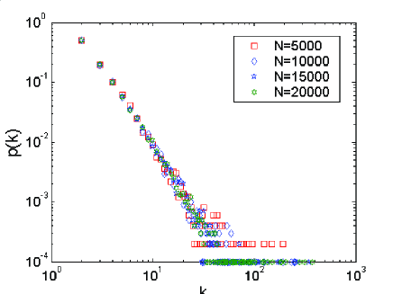
Figure 1: Degree distribution of MRGN, with $N=20000$ (hexagons), $N=15000$ (pentagons), $N=10000$ (diamonds) and $N=5000$ (squares). In this figure, $p(k)$ denotes the probability of the number of nodes with degree $k$ in the network. The power-law degree distribution exponent $\gamma$ of the four probability density function are $\gamma_{25000}=2.88\pm 0.02$, $\gamma_{20000}=2.88\pm 0.05$, $\gamma_{15000}=2.86\pm 0.06$ and $\gamma_{10000}=2.85\pm 0.02$

As we have mentioned above, the degree distribution is one of the most important statistical characteristics of networks. The average distance is also one of the most important parameters to measure the efficiency of communication network. The average distance $L$ of the network is defined as the mean distance over all pairs of nodes. The average distance plays a significant role in measuring the transmission delay. Marked each node of the network according to the time when the node is added to the network. Firstly, we give the following lemma M1 .

Lemma 1 For any two nodes $i$ and $j$, each shortest path from $i$ to $j$ does not pass through any nodes $k$ satisfying that $k>{\rm max}\{i,j\}$.

Proof. Denote the shortest path from node $i$ to $j$ of length $n+1$ by $i\rightarrow x^{1}\rightarrow x^{2}\cdots\rightarrow x^{n}\rightarrow j$($SP_{ij}$), where $n>0$. Suppose that $x^{k}={\rm max}\{x^{1},x^{2},\cdots,x^{n}\}$, if $k\leq{\rm max}\{i,j\}$, then the conclusion is true.

Then we prove the case that $k>{\rm max}\{i,j\}$ would not come forth. Suppose the edge $E_{y_{1}y_{2}}$ is selected when node $x_{k}$ is added. If $k>{\rm max}\{i,j\}$, neither node $i$ nor node $j$ is belong to the $E_{y_{1}y_{2}}$. Hence the path from $i$ to $j$ passing through $x^{k}$ must enter and leave $E_{y_{1}y_{2}}$. Assume that the path enter $E_{y_{1}y_{2}}$ by node $y_{1}$ and leave from node $y_{2}$, then there exists a path of $SP_{ij}$ from $y_{1}$ to $y_{2}$ passing through $x^{k}$, which is longer than the direct path $y_{1}\rightarrow y_{2}$. The youngest node must be either $i$ or $j$ when $SP_{ij}$ is the shortest path.

Denote $d(i,j)$ as the distance between node $i$ and node $j$. Let $\sigma(N)$ represent the total distance $\sigma(N)=\sum_{1\leq i<j\leq N}d(i,j)$. The average distance of MRGN with order $N$, denoted by $L(N)$, is defined as following

$$L(N)=\frac{2\sigma(N)}{N(N-1)}.$$ (7)

According to Lemma 3.1, the node newly added in the network will not affect the distance between old nodes. Hence we have

$$\sigma(N+1)=\sigma(N)+\sum^{N}_{i=1}d(i,N+1).$$ (8)

Assume that the $(N+1)$th node is add to the edge $E_{y_{1}y_{2}}$, then Equ.(8) can be written as

$$\sigma(N+1)=\sigma(N)+N+\sum^{N}_{i=1}D(i,y).$$ (9)

where $D(i,y)={\rm min}\{d(i,y_{1}),d(i,y_{2})\}$. Let a single node $y$ represent the $E_{y_{1}y_{2}}$ continuously, then we have the following equation

$$\sigma(N+1)=\sigma(N)+N+\sum_{i=\Lambda}d(i,y),$$ (10)

where the node set $\Lambda=\{1,2,\cdots,N\}-\{y_{1},y_{2}\}$ have $(N-2)$ members. The sum $\sum_{i=\Lambda}d(i,y)$ can be considered as the distance from each node of the network to node $y$ in MRGN with order $N-1$. Approximately, the sum $\sum_{i=\Lambda}d(i,y)$ is equal to $L(N-1)$. Hence we have

$$\sum_{i=\Lambda}d(i,y)\approx(N-2)L(N-1)$$ (11)

Because the average distance $L(N)$ increases monotonously with $N$, this yields

$$(N-2)L(N-1)=(N-2)\frac{2\sigma(N-1)}{(N-1)(N-2)}<\frac{2\sigma(N)}{N-1}.$$ (12)

Then we can obtain the inequality

$$\sigma(N+1)<\sigma(N)+N+\frac{2\sigma(N)}{N-1}.$$ (13)

Enlarge $\sigma(N)$, then the upper bound of the increasing tendency of $\sigma(N)$ will be obtained by the following equation

$$\frac{d\sigma(N)}{dN}=N+\frac{2\sigma(N)}{N-1}.$$ (14)

This leads to the following solution

$$\sigma(N)={\rm log}(N-1)(N-1)^{2}+C_{1}(N-1)^{2}-(N-1).$$ (15)

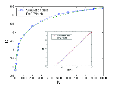
Figure 2: The dependence between the average distance $L$ and the order $N$ of MRGN. One can see that $L$ increases very slowly as $N$ increases. The inset exhibits the curve where $L$ is considered as a function of ${\rm ln}N$, which is fitted by a straight line. The curve is above the fitting line when $N$ is small($2000\leq N\leq 7000$) and under the fitting line when $N$ is large($N\geq 8000$), which indicates that the increasing tendency of $L$ can be approximated as ${\rm ln}N$ and in fact a little slower than ${\rm ln}N$. All the data are obtained by 10 independent simulations.

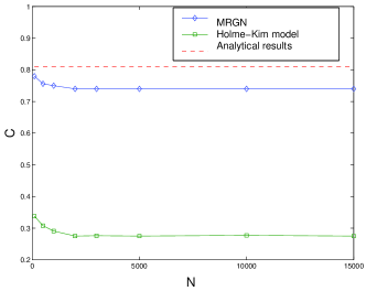
Figure 3: The clustering coefficient of MRGN(red diamonds) and Holme-Kim networks(green squares). In this figure, one can find that the clustering coefficient of MRGN is almost a constant a little smaller than 0.75. The red line represents the analytic result 0.81. It is clear that, the clustering coefficient of Holme-Kim networks is much smaller than that of MRGN.

By means of the theoretic approximate calculation, we prove that the increasing tendency of $L(N)$ is a little slower than ln$N$. In Fig 3, we report the simulation results on average distance of MRGN, which agree with the analytic result.

The small-world effect consists of two properties: large clustering coefficient and small average distance. The clustering coefficient, denoted by $C$, is defined as $C=\sum_{i=1}^{N}\frac{C_{i}}{N}$, where $C_{i}$ is the clustering coefficient for any arbitrary node $i$. $C_{i}$ is

$$C_{i}=\frac{2E(i)}{k_{i}(k_{i}-1)},$$ (16)

where $E(i)$ is the number of edges in the neighbor set of the node $i$, and $k_{i}$ is the degree of node $i$. When the node $i$ is added to the network, it is of degree 2 and $E(i)=1$. If a new node is added to be a neighbor of $i$ at some time step, $E(i)$ will increase by one since the newly added node will link to one of the neighbors of node $x$. Therefore, in terms of $k_{i}$ the expression of $E(i)$ can be written as following

$$E(i)=1+(k_{i}-2)=k_{i}-1.$$ (17)

Hence, we have that

$$C_{i}=\frac{2(k_{i}-1)}{k_{i}(k_{i}-1)}=\frac{2}{k_{i}}.$$ (18)

This expression indicates that the local clustering scales as $C_{i}\sim k^{-1}$. It is interesting that a similar scaling has been observed in pseudofractal web M8 and several real-life networks M9 . Consequently, we have

$$C=\frac{2}{N}\sum^{N}_{i=1}\frac{1}{k_{i}}.$$ (19)

Since the degree distribution is $p(k)=c_{1}k^{-3}$, where $k=2,3,\cdots,k_{\rm max}$. The average clustering coefficient $C$ can be rewritten as

$$C=\sum_{k=2}^{k_{\rm max}}\frac{2}{N}\frac{Np(k)}{k}=2c_{1}\sum_{k=2}^{k_{\rm max}}k^{-4}.$$ (20)

For sufficient large $N$, $k_{max}\gg 2$. The parameter $c_{1}$ satisfies the normalization equation

$$\sum_{k=2}^{k_{\rm max}}p(k)dk=1.$$ (21)

It can be obtain that $c_{1}=4.9491$ and $C=2\times 4.9491\times\sum_{k=2}^{k_{\rm max}}k^{-4}=0.8149$. From Fig. 4, we can get that the analytical average clustering coefficient deviance the real value a little. Because the analytic one is obtained when the time step $t\rightarrow\infty$ and the simulation result is obtained when the time step $t$ is finite. The other reason is that simulation result $\gamma$ of the degree distribution deviant $3$ a little, which is caused the finite network size. However, the most important reason lies in the hypothesis (4) that there are no correlations between all nodes. The demonstration exhibits that most real-life networks have large clustering coefficient no matter how many nodes they have. That is agree with the case of MRGN but conflict with the case of BA networks, thus MRGN may be more appropriate to mimic the reality.

In summary, we have introduced a simple iterative algorithm for constructing MRGN. The networks have very large clustering coefficients and very small average distance, which satisfy many real networks characteristics, such as the technological and social networks. After the newly added node connect to the first node $i$, it connect to the neighbor node of node $i$ preferentially. They are not only the scale-free networks, but also small-world networks. The results imply the following conclusion: if there are no correlation between all node and the new node adds to the network in two step, whether the second step is random or preferential, the degree distribution would be power-law and the exponent is 3. We have computed the analytical expressions for the degree distribution and clustering coefficient. Since most real-life networks are both scale-free and small-world networks, MRGN may perform better in mimicking reality. Further work should focus on the information flow and the epidemic spread on MRGN.

This work has been supported by the Chinese Natural Science Foundation of China under Grant Nos. 70431001 and 70271046.

References

- (1) Watts D J and Strogatz S H 1998 Nature 393 440
- (2) Barabsi A L and Albert R 1999 Science 286 509
- (3) Albert R and Barabási A L 2002 Rev. Mod. Phys. 74 47
- (4) Dorogovtsev S N and Mendes J F F 2002 Adv. Phys. 51 1079
- (5) Newmann M E J 2003 SIAM Rev. 45 167
- (6) Wang 2002 X F Int. J. Bifurcat. Chaos 12 885
- (7) Li W and Cai X 2004 Phys. Rev. E 69 046106
- (8) Wang R and Cai X 2005 Chin. Phys. Lett. 22 2715
- (9) Xu T et al 2004 Int. J. Mod. Phys. B 18 2599
- (10) Zhang P P et al 2005 Physica A 359 835
- (11) Li M H et al 2005 Physica A 350 643
- (12) Fang J Q and Liang Y 2005 Chin. Phys. Lett. 22 2719
- (13) Zhao F C et al 2005 Phys. Rev. E 72 046119
- (14) Yang H J et al 2004 Phys. Rev. E 69 066104
- (15) Liu J G et al 2005 Preprint arXiv: physics/0509183
- (16) Tadić B et al 2004 Phys. Rev. E 69 036102
- (17) Zhao L et al 2005 Phys. Rev. E 71 026125
- (18) Yan G et al 2005 Preprint arXiv: cond-mat/0505366
- (19) Yin C Y et al 2005 Preprint arXiv: physics/0506204
- (20) Pastor-Satorras R and Vespignani A 2001 Phys. Rev, Lett. 86 3200
- (21) Yan G et al 2005 Chin. Phys. Lett. 22 510.
- (22) Zhou T et al 2005 Preprint arXiv: physics/0508096
- (23) Motter A E and Lai Y -C 2002 Phys. Rev. E 66 065102
- (24) Goh K I et al 2003 Phys. Rev. Lett. 91 148701
- (25) Zhou T and Wang B -H 2005 Chin. Phys. Lett. 22 1072
- (26) Zhou T et al 2005 Phys. Rev. E 72 016139
- (27) Zhao M et al 2005 Preprint arXiv: cond-mat/0507221
- (28) Zhou T et al 2005 Preprint arXiv: cond-mat/0508368
- (29) Duan W Q et al 2005 Chin. Phys. Lett. 22 2137
- (30) Fan J et al 2005 Physica A 355 657
- (31) Valente A X C N et al 2004 Phys. Rev. Lett. 92 118702
- (32) Paul G et al 2004 Eur. Phys. J. B 38 187
- (33) Wang B et al 2005 Preprint arXiv:cond-mat/0509711
- (34) Wang B et al 2005 Preprint arXiv:cond-mat/0506725
- (35) Liu J G et al 2005 Mod. Phys. Lett. B 19 785
- (36) Liu J G et al 2005 Preprint arXiv:cond-mat/0509290
- (37) Zhou T et al 2005 Phys. Rev. E 71 046141
- (38) Andrade J S et al 2005 Phys. Rev. Lett. 94 018702
- (39) Comellas F et al 2004 Phys. Rev. E 69 037104
- (40) Comellas F and Sampels M 2002 Physica A 309 231
- (41) Zhang Z Z and Rong L L 2005 Preprint arXiv:cond-mat/0502591
- (42) Dorogovtsev S N et al 2001 Phys. Rev. E 63 062101
- (43) Holme P and Kim J 2002 Phys. Rev. E 65 065107
- (44) Dorogovtsev S N et al 2002 Phys. Rev. E 65 066122
- (45) Ravasz E and Barabsi A L 2003 Phys. Rev. E 67 026112
- (46) Jiang P Q et al 2005 Chin. Phys. Lett. 22 1285
- (47) Wang W X et al 2005 Phys. Rev. E 72 046140
- (48) Wang W X et al 2005 Phys. Rev. Lett. 94 188702
- (49) Zhu C P et al 2004 Phys. Rev. Lett. 92 218702