Observation of Brewster’s effect for transverse-electric electromagnetic waves in metamaterials: Experiment and theory

Abstract

We have experimentally realized Brewster’s effect for transverse-electric (TE) waves with metamaterials. In dielectric media, Brewster’s no-reflection effect arises only for transverse-magnetic (TM) waves. However, it has been predicted theoretically that Brewster’s effect arises for TE waves under the condition that the relative permeability $\mu_{\scriptsize\mbox{r}}$ is not equal to unity. We have designed an array of split ring resonators (SRRs) as a metamaterial with $\mu_{\scriptsize\mbox{r}}\neq 1$ using a finite-difference time-domain (FDTD) method. The reflection measurements were carried out in a 3-GHz region and the disappearance of reflected waves at a particular incident angle was confirmed.

Brewster’s no-reflection condition is one of the main features of the laws of reflection and refraction of electromagnetic waves at a boundary between two media. For a specific incident angle, known as the Brewster angle, the reflection wave vanishes. In dielectric media, this phenomenon exists only for transverse-magnetic (TM) waves (p waves), and not for transverse-electric (TE) waves (s waves). It is conveniently applied in optical instruments. One can generate completely polarized light from an unpolarized light source only with a glass plate. It can also be used to avoid the reflection losses at the surfaces of optical components. The Brewster window of the discharge tube in gaseous lasers is a typical example.

For a plane electromagnetic wave incident on the plane boundary between medium 1 and medium 2, the amplitude reflectivities of TE and TM waves are given by the Fresnel formulae:

$$r_{\scriptsize\mbox{TE}}=\frac{\sin{(\theta_{\scriptsize\mbox{t}}-\theta_{\scriptsize\mbox{i}})}}{\sin{(\theta_{\scriptsize\mbox{t}}+\theta_{\scriptsize\mbox{i}})}},\quad r_{\scriptsize\mbox{TM}}=\frac{\tan{(\theta_{\scriptsize\mbox{i}}-\theta_{\scriptsize\mbox{t}})}}{\tan{(\theta_{\scriptsize\mbox{i}}+\theta_{\scriptsize\mbox{t}})}},$$ (1)

where $\theta_{\scriptsize\mbox{i}}$ and $\theta_{\scriptsize\mbox{t}}$ are the angles of incidence and transmission, respectively Hecht (1998). The numerators in Eq. (1) cannot vanish because $\theta_{\scriptsize\mbox{i}}$ is not equal to $\theta_{\scriptsize\mbox{t}}$. However, $r_{\scriptsize\mbox{TM}}$ can vanish because $\tan{(\theta_{\scriptsize\mbox{i}}+\theta_{\scriptsize\mbox{t}})}$ diverges to infinity when $(\theta_{\scriptsize\mbox{i}}+\theta_{\scriptsize\mbox{t}})$ is equal to $\pi/2$.

Physically, Brewster’s phenomena can be understood as follows. The direction of the induced electric dipole in medium 2 is perpendicular to the wavevector therein. With regard to TM waves, the dipole lies in the plane of incidence. A linearly vibrating dipole radiates transversally and cannot emit radiation in the direction of the vibration. This direction coincides with the wavevector of the reflected wave when the Brewster condition is satisfied. The oscillating dipoles in the medium 2 do not send any waves in the direction of the reflection. On the other hand, with regard to TE waves, each dipole is perpendicular to the plane of incidence and emits waves isotropically in the plane. Therefore, no special angles exist for TE waves. (The dipole model also explains the sign change in the amplitude reflectivity when the angle is changed through the Brewster angle.)

Brewster’s effect in dielectric media exists only for TM waves, and not for TE waves. This asymmetry results from the assumption that the relative permeability $\mu_{\scriptsize\mbox{r}}$ is almost unity for higher frequencies, such as microwaves and light waves. Each medium is characterized only by its relative permittivity $\varepsilon_{\scriptsize\mbox{r}}$. The assumption that is used in deriving Eq. (1) is quite reasonable because for common materials, any kind of magnetic response is frozen in high frequency regions. However, the assumption must be reconsidered for metamaterials, for which both $\varepsilon_{\scriptsize\mbox{r}}$ and $\mu_{\scriptsize\mbox{r}}$ can be changed significantly from unity. Brewster’s effects in general cases such as magnetic, anisotropic, and chiral madia have been studied Doyle (1980); Lakhtakia (1992); Futterman (1995) and no-reflection phenomena for other than TM waves have been predicted. The use of metamaterials for verifying these generalized Brewster effects have been suggested Leskova et al. (2001, 2003); Fu et al. (2005). In this Letter, we demonstrate the Brewster effect for TE waves in magnetic metamaterials experimentally.

A metamaterial is composed of small conductive elements such as coils or rods, upon which currents are induced by the incident electric or magnetic fields. When their sizes and separations are significantly smaller than the wavelengths, the collection of elements can be viewed as a continuous medium. By utilizing resonant structures, both $\varepsilon_{\scriptsize\mbox{r}}$ and $\mu_{\scriptsize\mbox{r}}$ could be significantly shifted from unity. In particular, a medium with $\varepsilon_{\scriptsize\mbox{r}}<0$ and $\mu_{\scriptsize\mbox{r}}<0$ attracts attention because of its peculiar behaviors owing to the negative index of refraction $n=\sqrt{\varepsilon_{\scriptsize\mbox{r}}}\sqrt{\mu_{\scriptsize\mbox{r}}}=-\sqrt{|\varepsilon_{\scriptsize\mbox{r}}\mu_{\scriptsize\mbox{r}}|}$ Veselago (1968). Negative refraction has been experimentally confirmed in microwave and terahertz regions Shelby et al. (2001); Parazzoli et al. (2003); Houck et al. (2003).

An artificial medium with $\varepsilon_{\scriptsize\mbox{r}}=1$, $\mu_{\scriptsize\mbox{r}}\neq 1$, which is a dual of normal dielectric materials, $\varepsilon_{\scriptsize\mbox{r}}\neq 1$, $\mu_{\scriptsize\mbox{r}}=1$, can be designed. Magnetic dipoles are induced by the magnetic field of the incident wave. Repeating the discussion with the dipole model, one can conclude that Brewster’s effect can be observed for TE waves in the case of such magnetic metamaterials.

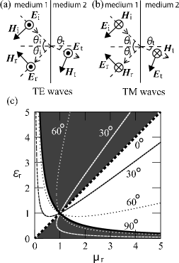
Figure 1: The relation between electric and magnetic fields for (a) TE waves and (b) TM waves. (c) Brewster condition for media with relative permittivity $\varepsilon_{\scriptsize\mbox{r}}$ and relative permeability $\mu_{\scriptsize\mbox{r}}$. Brewster conditions for TE waves and TM waves exist in the unshaded and shaded areas, respectively. The curves represent the contour lines of the Brewster angles.

We assume that medium 1 is a vacuum and medium 2 is a medium with $\varepsilon_{\scriptsize\mbox{r}}$ and $\mu_{\mathrm{r}}$. The amplitude reflectivities for TE waves and TM waves are expressed as follows:

$$r_{\scriptsize\mbox{TE}}=\frac{Z_{\scriptsize\mbox{r}}\cos\theta_{\scriptsize\mbox{i}}-\cos\theta_{\scriptsize\mbox{t}}}{Z_{\scriptsize\mbox{r}}\cos\theta_{\scriptsize\mbox{i}}+\cos\theta_{\scriptsize\mbox{t}}},\quad r_{\scriptsize\mbox{TM}}=\frac{\cos\theta_{\scriptsize\mbox{i}}-Z_{\scriptsize\mbox{r}}\cos\theta_{\scriptsize\mbox{t}}}{\cos\theta_{\scriptsize\mbox{i}}+Z_{\scriptsize\mbox{r}}\cos\theta_{\scriptsize\mbox{t}}},$$ (2)

where $Z_{\scriptsize\mbox{r}}=\sqrt{\mu_{\scriptsize\mbox{r}}/\varepsilon_{\scriptsize\mbox{r}}}$ is the normalized wave impedance of medium 2 Hecht (1998). The incident angle $\theta_{\scriptsize\mbox{i}}$ and the transmitted angle $\theta_{\scriptsize\mbox{t}}$ are related by Snell’s law $\sin\theta_{\scriptsize\mbox{i}}/\sin\theta_{\scriptsize\mbox{t}}=n$ with $n=\sqrt{\varepsilon_{\scriptsize\mbox{r}}}\sqrt{\mu_{\scriptsize\mbox{r}}}$. The no-reflection conditions, $r_{\scriptsize\mbox{TE}}=0$ or $r_{\scriptsize\mbox{TM}}=0$, can be written as follows:

$$0\leq\sin^{2}\theta_{\scriptsize\mbox{i}}=\frac{\alpha^{2}-n^{2}}{\alpha^{2}-1}\leq 1,$$ (3)

where $\alpha=\mu_{\scriptsize\mbox{r}}$ for TE waves and $\alpha=\varepsilon_{\scriptsize\mbox{r}}$ for TM waves. Theoretical derivations of the Brewster angles for general media have been presented in previous works Lakhtakia (1992); Futterman (1995); Leskova et al. (2001, 2003); Fu et al. (2005). With this equation, the Brewster angle can be determined for a given pair, $(\mu_{\scriptsize\mbox{r}},\varepsilon_{\scriptsize\mbox{r}})$. In Fig. 1 (c), the Brewster angles are plotted parametrically on the $(\mu_{\scriptsize\mbox{r}},\varepsilon_{\scriptsize\mbox{r}})$-plane. Based on the inequalities of Eq. (3), we see that the Brewster angle for TM waves exists only in the shaded area in Fig. 1 (c). By exchanging the roles of $\varepsilon_{\scriptsize\mbox{r}}$ and $\mu_{\scriptsize\mbox{r}}$, we obtain the Brewster condition for TE waves as indicated by the unshaded area in Fig. 1 (c).

Figure 2: (a) Split ring resonator. $r$ is the average radius of two rings; $w$, the width of the ring; $d$, the distance between the two rings; $t$, the thickness of the ring. (b) SRR used in the FDTD analysis.

Figure 3: Complex relative permittivity $\varepsilon_{\scriptsize\mbox{r}}$ and complex relative permeability $\mu_{\scriptsize\mbox{r}}$ versus frequency for the SRR array. The SRRs in Fig. 2 (b) are placed every $4.4\,{\mu\Omega\mathrm{mm}}$ in both the $E$ direction and the $H$ direction to form a 2D array. The array is a monolayer in the $k$ direction. The conductivity of the ring is $1.0\times 10^{8}\,{\mu\Omega\mathrm{S/m}}$. $R_{\scriptsize\mbox{min}}/R_{0}$ is very small in the frequency region and is represented by the arrow marked with an asterisk.

It is apparent that Brewster’s effect arises only for TM waves in normal media ($\mu_{\scriptsize\mbox{r}}=1$). However, for a medium with $\mu_{\scriptsize\mbox{r}}\neq 1$, the Brewster condition for TE waves can be realized. For a given $\mu_{\scriptsize\mbox{r}}\gtrless 1$, when $1/\mu_{\scriptsize\mbox{r}}\lessgtr\varepsilon_{\scriptsize\mbox{r}}\lessgtr\mu_{\scriptsize\mbox{r}}$ is satisfied, there exists a Brewster angle for TE waves. In other words, the medium must be more magnetic, rather than electric, in order to realize the Brewster condition for TE waves.

We consider an array of split ring resonators (SRRs), as shown in Fig. 2 (a). It serves as a magnetic medium with $\mu_{\scriptsize\mbox{r}}\neq 1$ in microwave regions Pendry et al. (1999). Each SRR functions as a series resonant circuit formed by the ring inductance and inter-ring capacitance. When we apply time-varying magnetic fields through the ring, a circular current around the ring is induced near the resonance frequency so that it produces a magnetic moment. Owing to the resonant structure, the effective permeability $\mu_{\scriptsize\mbox{r}}$ could be significantly different from unity.

We calculate the relative complex permittivity $\varepsilon_{\scriptsize\mbox{r}}$ and permeability $\mu_{\scriptsize\mbox{r}}$ of the SRR array using a finite-difference time-domain (FDTD) method Taflove and Hagness (2005). We consider a rectangular SRR, as shown in Fig. 2 (b), for the purpose of simplicity in calculation. Assuming that a plane wave is incident on the SRR array, we analyzed the charge distribution and the induced current, from which the electric and magnetic dipole moments originate. The permittivity $\varepsilon_{\scriptsize\mbox{r}}$ (permeability $\mu_{\scriptsize\mbox{r}}$) can be derived from an electric (magnetic) dipole moment of a single SRR and the density of the SRRs Smith et al. (2000).

Figure 3 shows $\varepsilon_{\scriptsize\mbox{r}}$ and $\mu_{\scriptsize\mbox{r}}$ as a function of frequency $f$. The real parts of $\varepsilon_{\scriptsize\mbox{r}}$ and $\mu_{\scriptsize\mbox{r}}$ are related to the dispersive or refractive properties of metamaterials, and the imaginary parts are related to the losses or absorption. As seen in Fig. 3, the permittivity can be regarded as unity for any frequency, and ${\rm Re}(\mu_{\scriptsize\mbox{r}})$ and ${\rm Im}(\mu_{\scriptsize\mbox{r}})$ can be approximated by the Lorentz dispersion and absorption functions. The ratio of the maximum value of $\left|\varepsilon_{\scriptsize\mbox{r}}(f)-1\right|$ to that of $\left|\mu_{\scriptsize\mbox{r}}(f)-1\right|$ is less than $2\,\%$. The electric response of SRR is much weaker than the magnetic response especially for the electric field in the direction of symmetric axis of reflection. This fact agrees with previous studies Gay-Balmaz and Martin (2002); Katsarakis et al. (2004). The SRR array functions as a magnetic medium with finite losses. We also found that the LC circuit model is helpful in the estimation of the resonance frequency.

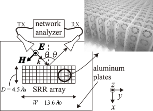
Figure 4: Schematic diagram of the reflectivity measurement system. Measurement is performed in a 2D waveguide composed of two aluminum plates. The separation between two aluminum plates is $38\,{\mu\Omega\mathrm{mm}}(=0.38\lambda_{0})$.

The reflectivity at the Brewster angle for the SRR array, unlike an ideal medium without losses, has a nonzero value due to the dissipation. If the dispersive property of the magnetic medium dominates the dissipation, we can detect a significant depression in the power reflectivity around the Brewster angle. In order to estimate the magnitude of the depression, we introduce the ratio of the minimum power reflectivity $R_{\scriptsize\mbox{min}}$ to the power reflectivity for normal incidence, $R_{0}$. The lesser the ratio $R_{\scriptsize\mbox{min}}/R_{0}$, the more easily we can detect Brewster’s effect in the experiments. From the calculation by the FDTD method, we find that the ratio $R_{\scriptsize\mbox{min}}/R_{0}$ reduces in a narrow region below the resonance frequency, which is indicated by the arrow marked with an asterisk in Fig. 3, and the Brewster condition for the TE wave could easily be detected.

Figure 5: (a) Power reflectivity of the SRR array at $f=2.6001\,{\mu\Omega\mathrm{GHz}}$ as a function of $\theta$. (b) Measured (solid circle) and calculated (dashed line) Brewster angles versus frequency.

A power-reflectivity measurement system as shown in Fig. 4, is used to observe Brewster’s effect for the TE waves with an SRR array.

The SRRs are formed on printed circuit boards. To facilitate easy preparation, the parameters are chosen as $r=4.0\,{\mu\Omega\mathrm{mm}},~{}w=0.61\,{\mu\Omega\mathrm{mm}},~{}d=0.48\,{\mu\Omega\mathrm{mm}}$, and $t=35\,{\mu\Omega\mathrm{um}}$. From a simplified LC circuit model, the resonance frequency is estimated to be $3.04\,{\mu\Omega\mathrm{GHz}}$; this corresponds to the wavelength in a vacuum, $\lambda_{0}=9.9\,{\mu\Omega\mathrm{cm}}$.

We set two aluminum plates ($1\,{\mu\Omega\mathrm{m}}\times 1.5\,{\mu\Omega\mathrm{m}}$) parallel to each other to form a two-dimensional waveguide, in which horn antennas and an SRR array are inserted. The separation between the two plates is $38\,{\mu\Omega\mathrm{mm}}(=0.38\lambda_{0})$. In this waveguide, the electric field is perpendicular to the plates, and the electromagnetic field becomes uniform along the $z$ direction. Thus only TE waves can be propagated. We note that the direction of electric field does not change for the change of the incident angle $\theta$ and fixed to the direction of the minimum electric response of the SRR array.

The unit cell size of an SRR array must be significantly smaller than $\lambda_{0}$; therefore, we arranged the SRRs every $1.4\,{\mu\Omega\mathrm{cm}}(=0.14\lambda_{0})$ in the $x$ and $y$ directions and $1.3\,{\mu\Omega\mathrm{cm}}(=0.13\lambda_{0})$ in the $z$ direction. The direction of $H$ varies in the $xy$ plane because the power reflectivity is measured for various incident angles $\theta$. We arranged the SRRs orthogonally to make the response of the SRR array isotropic. The dimension of the SRR array is $(W,D,T)=(135\,{\mu\Omega\mathrm{cm}},45\,{\mu\Omega\mathrm{cm}},38\,{\mu\Omega\mathrm{mm}})=(13.6\lambda_{0},4.5\lambda_{0},0.38\lambda_{0})$. In order to ensure an extended boundary, we set the width $W$ to be significantly larger than $\lambda_{0}$. We made the depth $D$ sufficiently large so that the influence of the back side reflection can be avoided.

First, we measured the transmissivity of the SRR array in order to determine the resonance frequency $f_{0}$, which was found to be $2.65\,{\mu\Omega\mathrm{GHz}}$; it was $12.8\,\%$ smaller than the value calculated with the LC circuit model.

We used a network analyzer as the microwave generator and detector. We connected a horn antenna (the aperture size is $15\,{\mu\Omega\mathrm{cm}}\times 3.4\,{\mu\Omega\mathrm{cm}}$) to the transmitting port of the network analyzer in order to transmit a slowly diverging beam. We use another horn antenna connected to the receiving port in order to receive the plane wave reflected at the boundary. Only the plane wave propagating normal to the antenna aperture can be coupled to the receiver. We always set the direction of the receiving horn antenna such that a plane wave reflected with a reflection angle equal to the incident angle is detected.

We measured the $\theta$ dependence of the power reflectivity for a fixed frequency. One of the results is shown in Fig. 5 (a). Compared with the case of perfect reflection, the reflectivity decreases by more than $27\,{\mu\Omega\mathrm{dB}}$ in the vicinity of $\theta=60^{\circ}$, which corresponds to the Brewster angle for TE waves.

We measured the frequency dependence of the Brewster angle. The result is shown in Fig. 5 (b) (solid circles). The Brewster angles could be determined only in a limited region just below the resonance frequency. In this region, the measured Brewster angles increase with the frequency. We calculated the frequency dependence of the Brewster angles from Eq. (2) by assuming $\varepsilon_{\scriptsize\mbox{r}}(f)=1$ and $\mu_{\scriptsize\mbox{r}}(f)=1-F/(f^{2}+{\mathrm{i}}\gamma f-f_{0}^{2})$, where $f_{0}=2.65\,{\mu\Omega\mathrm{GHz}}$ is the resonance frequency that is previously determined by the absorption measurement. By fitting the calculated values to the measured values, we fixed the parameters $F$ and $\gamma$. The calculated angle is shown as the dashed line in Fig. 5 (b). It increases with frequency; this is in agreement with the experimental results.

As previously discussed, we can observe the Brewster angles only in a limited frequency region. It should be noted that in actual experiments, the reflectivity varies somewhat erratically due to the interference of spurious waves or other reasons, and the dip in reflectivity can be detected only for the cases where $R_{\scriptsize\mbox{min}}/R_{0}$ is sufficiently small. In the other on-resonance frequency regions, $R_{\scriptsize\mbox{min}}$ cannot be sufficiently small due to the absorption losses. On the other hand, $R_{0}$ reduces in the off-resonance regions.

In conclusion, we observed Brewster’s effect for TE waves, which had previously never been observed for normal dielectric media. We need a medium whose $\mu_{\scriptsize\mbox{r}}$ is not equal to unity. We have used a metamaterial composed of SRRs in order to achieve a magnetic medium in a microwave region. This is a good example of the use of metamaterials. In terms of the parameter space $(\mu_{\scriptsize\mbox{r}},\varepsilon_{\scriptsize\mbox{r}})$, by introducing metamaterials, the rigid condition of $\varepsilon_{\scriptsize\mbox{r}}>0$, $\mu_{\scriptsize\mbox{r}}=1$ can be eliminated. The restrictions $\varepsilon_{\scriptsize\mbox{r}}>0$ and $\mu_{\scriptsize\mbox{r}}>0$ can also be eliminated. The working range of metamaterials presently extends from microwaves to terahertz or even to optical regions. In the near future, we may be able to fabricate a Brewster window for TE light.

This research was supported by the 21st Century COE Program No. 14213201.

References

- Hecht (1998) E. Hecht, Optics (Addison-Wesley, 1998), 3rd ed.
- Doyle (1980) W. T. Doyle, Am. J. Phys. 48, 643 (1980).
- Lakhtakia (1992) A. Lakhtakia, Z. Naturforsch. A 47, 921 (1992).
- Futterman (1995) J. Futterman, Am. J. Phys. 63, 471 (1995).
- Leskova et al. (2001) T. A. Leskova, A. A. Maradudin, and I. Simonsen, Proc. SPIE 4447, 6 (2001).
- Leskova et al. (2003) T. A. Leskova, A. A. Maradudin, and I. Simonsen, Proc. SPIE 5189, 22 (2003).
- Fu et al. (2005) C. Fu, Z. M. Zhang, and P. N. First, Appl. Opt. 44, 3716 (2005).
- Veselago (1968) V. G. Veselago, Sov. Phys. Usp. 10, 509 (1968).
- Shelby et al. (2001) R. A. Shelby, D. R. Smith, and S. Schultz, Science 292, 77 (2001).
- Parazzoli et al. (2003) C. G. Parazzoli, R. B. Greegor, K. Li, B. E. C. Koltenbah, and M. Tanielian, Phys. Rev. Lett. 90, 107401 (2003).
- Houck et al. (2003) A. A. Houck, J. B. Brock, and I. L. Chuang, Phys. Rev. Lett. 90, 137401 (2003).
- Pendry et al. (1999) J. Pendry, A. Holden, D. Robbins, and W. Stewart, IEEE Trans. Microwave Theory Tech. 47, 2075 (1999).
- Taflove and Hagness (2005) A. Taflove and S. C. Hagness, Computational electrodynamics: the finite-difference time-domain method (Artech House, 2005), 3rd ed.
- Smith et al. (2000) D. R. Smith, D. C. Vier, N. Kroll, and S. Schultz, Appl. Phys. Lett. 77, 2246 (2000).
- Gay-Balmaz and Martin (2002) P. Gay-Balmaz and O. J. F. Martin, J. Appl. Phys. 92, 2929 (2002).
- Katsarakis et al. (2004) N. Katsarakis, T. Koschny, M. Kafesaki, E. N. Economou, and C. M. Soukoulis, Appl. Phys. Lett. 84, 2943 (2004).