Monte Carlo simulation of melting transition on DNA nanocompartment

Abstract

DNA nanocompartment is a typical DNA-based machine whose function is dependent of molecular collective effect. Fundamental properties of the device have been addressed via electrochemical analysis, fluorescent microscopy, and atomic force microscopy. Interesting and novel phenomena emerged during the switching of the device. We have found that DNAs in this system exhibit a much steep melting transition compared to ones in bulk solution or conventional DNA array. To achieve an understanding to this discrepancy, we introduced DNA-DNA interaction potential to the conventional Ising-like Zimm-Bragg theory and Peyrard-Bishop model of DNA melting. To avoid unrealistic numerical calculation caused by modification of the Peyrard-Bishop nonlinear Hamiltonian with the DNA-DNA interaction, we established coarse-gained Monte Carlo recursion relations by elucidation of five components of energy change during melting transition. The result suggests that DNA-DNA interaction potential accounts for the observed steep transition.

$\textrm{Song Chang}^{1,\,2}$, $\textrm{Youdong Mao}^{1}$, $\textrm{Zhengwei Xie}^{2}$ $\textrm{Chunxiong Luo}^{1}$, $\textrm{Qi Ouyang}^{1,\,2,\,3}$
$\textrm{}^{1}$Laboratory of Biotechnology, School of Physics, Peking University, Beijing 100871, China
$\textrm{}^{2}$Center for Theoretical Biology, Peking University, Beijing 100871, China
$\textrm{}^{3}$To whom correspondence should be addressed.
E-mail: qi@pku.edu.cn

1.Introduction
Studies on the physical chemistry of DNA denaturation have been lasted for almost forty years [1-3]. In 1964, Lifson proposed that a phase transition exists in one-dimensional polymer structure. He introduced several pivotal concepts, like sequence partition function, sequence generating function, etc., and established a systematic method to calculate the partition function [1]. These allow us to derive important thermodynamic quantities of the system. In 1966, Poland and Scherage applied Lifson’s method to conduct research on amino acid and nucleic acid chains. They built Poland-Scherage (PS) model for calculating the sequence partition function and discussing the behavior of polymers in melting transitions.
Another excellent progress would be the building of Peyrard-Bishop (PB) model [4,5] for DNA chains. In PB model, the Hamiltonian of a single DNA chain, which is constructed by phonon calculations, is given so that we can obtain the system properties through statistical physics method. The PB model has introduced mathematical formula of stacking energy, as well as the kinetic energy and potential energy of each base pair. By theoretical calculation, one can show the entropy-driven transition that leads DNA to shift from ordered state to disorder one [6,7].
However, all these works have not involved the DNA-DNA interactions because the subject investigated is DNAs in bulk solution, and the interaction between them has ever been neglected. The main idea of this paper is to inspect the influence of collective effect on the DNA melting process, primarily motivated by the experiment results of DNA nanocompartment [8,9]. Under the enlightenment of Poland-Scherage model and Zimm-Bragg model [10], we simplify Peyrard-Bishop model to meet a reasonable Monte Carlo simulation by the elucidation of five components of energy changes during melting transition. The result shows that the melting temperature and transition duration depend on whether we take into account the DNA-DNA interactions among columnar assemblies of DNA.

2.Experiment
Recently, we found that specially designed DNA array can form a molecular cage on surfaces [8,9]. This molecular cage is switchable due to allosteric transformation driven by the collective hybridization of DNA. We named it ”active DNA nanocompartment (ADNC)”. Typical DNA motif designed to fabricate ADNC comprises two contiguous elements (inset to figure 1a): a double-stranded DNA (dsDNA) whose array is responsible for a compact membrane (figure 1a, right), and a single-stranded DNA (ssDNA) serving as skeleton supporting the dsDNA membrane, which is terminated on its 5 end by a surface linker such as an alkanethiol group that can be tethered to gold surface with a sulphur-gold bond [9] or an amino group that can be tethered to $\textrm{SiO}_{2}$ substrate with specific surface attachment chemistry [11]. Because the diameter of ssDNA is much smaller than that of dsDNA, a compartment with designable effective height (heff, $5\sim 50nm$, commensurate with the length of ssDNA skeleton) can form between the dsDNA membrane and substrate surface.
Since ADNC is reversibly switchable, it is able to encage molecules with suitable size. We name this phenomenon molecular encaging effect. Both electrochemical methods [12] and fluorescent microscopy are used to substantiate the molecular encaging effect and the reversibility of switching. Once the closed ADNC entraps some chemical reporters, the surface concentration ($\Gamma_{nc}$) of the encaged reporters can be determined by cyclic voltammetry or fluorescent microscopy. Figure 1b shows the isotherms of the molecular encaging effect for fluorescein ($\textrm{C}_{20}\textrm{H}_{10}\textrm{Na}_{2}\textrm{O}_{5}$). Figure 1c presents the melting curves of ADNC. Using the encaged molecules as indicator greatly sharpens the melting profiles for the perfectly complementary targets, and flattens denaturation profiles for the strands with a wobble mismatch. The observation shows that single-base mismatched strands are incapable of closing ADNC on surfaces. The result is highly consistent to our observation by electrochemical analysis [12]. These observations bring up an intriguing question: why the melting curves exhibit so steep transition compared to the case of DNA in bulk solutions or on a loosely packed microarray? We try to address this question in this paper.
Worthy of mention is that the steepness of melting transition is useful when the ADNC is applied to DNA detection [8,9]. First, it greatly enhances the discrepancy of perfect targets and single mismatches. This provides much enhanced specificity in DNA recognition, $100:1\sim 105:1$ of our system versus $2.7:1$ of conventional system. Second, more sensitivity is obtained with optimally decreased ambiguity. Therefore, the clarification of the origin of the steep shape should help us to further extend the experience to related fields or generate new techniques.

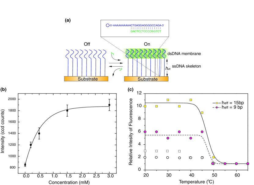
Figure 1: (a) Schematic drawing of a dual-state ADNC. By adding or removing ’fuel’ strands (shorter segment), the ADNC can be switched between on (right) and off (left) state. Inset, a typical sequence used to fabricate ADNC. The ’fuel’ strands is a segment of human p53 gene containing one site of most frequent mutation. (b) Isotherms of $\Gamma$ for fluorescein encaged in a closed ADNC ($h_{eff}=15bp$). The isotherm fits well to the Langmuir model: $x/\Gamma_{nc}=(1/\Gamma_{nc,max})x+(1/K\Gamma_{nc,max})$, where $x$ is the concentration of the reporter and $K$ is the association constant per site, $\Gamma_{nc}$ the surface concentration of encaged molecules. (c) Melting curves using the encaged fluorescein molecules as indicators. Filled circles or squares are corresponding to perfect complementary strands, and hollow circles or squares to single-base mismatched strands. The unit of relative intensity of fluorescein is defined as the light intensity of $5\mu l\,10nM$ fluorescein on a spot size with $5mm$ diameter. Inset shows the length of the ssDNA skeleton of nanocompartment and the complementary type. The background noise is within $1$ unit.

3.Modeling
Taking into account the directional specificity of the hydrogen bonds, the Hamiltonian of a single DNA chain is obtained as following form according to PB model [4-6],

$$H_{y}=\sum_{n}\bigg{[}\frac{1}{2}m\dot{y_{n}}^{2}+w(y_{n},y_{n-1})+V(y_{n})\bigg{]}$$ (1)

where the $y_{n}$ is the component of the relative displacement of bases along the direction of hydrogen bond. The stacking energy $w(y_{n},y_{n-1})$ corresponds to the interaction between neighboring base pair in one DNA chain

$$w(y_{n},y_{n-1})=\frac{k}{2}\bigg{[}1+\rho e^{-\alpha(y_{n}+y_{n-1})}\bigg{]}(y_{n}-y_{n-1})^{2}$$ (2)

The Morse potential describes the potential for the hydrogen bonds

$$V=D(e^{-\alpha y}-1)^{2}$$ (3)

However, in this study, the Hamiltonian in equation (1) is not sufficient; it neglects the structure of close-packing of DNA in ADNC. In our system, one should take into account the interactions between the nearest neighboring molecules [13,14]. To model the interaction, one envisions the molecules as rigid cylinders, carrying helical and continuous line charges on their surfaces. Each DNA duplex carries the negative charge of phosphates plus a compensating positive charge from the adsorbed counterions. Let $0<\theta<1$ be the degree of charge compensation, $f_{1}$, $f_{2}$ and $f_{3}$ the fractions of condensed counterions in the minor and major grooves ($f_{1}+f_{2}+f_{3}=1$). The mobile counterions in solution screen the Coulomb interactions between the two molecules, causing at large separations an exponential decay of the latter with the Debye screening length $\kappa^{-1}$. The solvent is accounted for by its dielectric constant $\varepsilon$. The structural parameters of B-DNA are half azimuthal width of the minor groove $\tilde{\phi_{s}}\approx 0.4\pi$ , pitch $H\approx 34\textrm{\AA}$($g=2\pi/H$), and hard-core radius $a=9\textrm{\AA}$. We take the following form for the pair interaction potential [15-18]:

$$u(R,\phi) = u_{0}\sum_{n=-\infty}^{\infty}\bigg{[}f_{1}\theta+(-1)^{n}f_{2}\theta-(1-f_{3}\theta)\cos(n\tilde{\phi_{s}})\bigg{]}^{2}$$ (4)

$$\times\frac{(-1)^{n}\cos(ng\Delta z)K_{0}(\kappa_{n}R)-\Omega_{n,n}(\kappa_{n}R,\kappa_{n}a)}{(\kappa_{n}/\kappa)^{2}[K^{\prime}_{n}(\kappa_{n}a)]^{2}}$$

where $R(>2a)$ is the distance between the two parallel DNA molecules, $\Delta z$ a vertical displacement, equivalent to a ”spin angle” $\phi=gz$. Here, $u_{0}=8\pi\sigma^{2}/\varepsilon\kappa^{2}$ (about $2.9k_{B}T/\textrm{\AA}$ at physiological ionic strength), and $\kappa_{n}=\sqrt{\kappa^{2}+n^{2}g^{2}}$. $\Omega_{n,m}(x,y)$ is given by

$$\Omega_{n,m}(x,y)=\sum_{j=-\infty}^{\infty}\bigg{[}K_{n-j}(x)K_{j-m}(y)\frac{I^{\prime}_{j}(y)}{K^{\prime}_{j}(y)}\bigg{]}$$ (5)

with the modified Bessel functions $K_{n}(x)$ and $I_{j}(y)$. The primes denote derivatives. The sum rapidly converges, and it can be truncated after $|n|=2$. Since $\kappa_{n}R>3$ and $g\sim\kappa$, each of the terms in the sum decreases exponentially at increasing $R$ with the decay length $\kappa_{n}^{-1}\propto 1/n$.
Figure 2 present a scheme of interaction between two neighboring columnar DNA molecules charged with counterions on its surface. The distance between two DNA columns in our simulation is about $30\textrm{\AA}$ and the helical pitch of DNA molecule is about $36\textrm{\AA}$. For brevity, we take the mean-field approximation that the pair interactions mainly exist between charges in the same height.

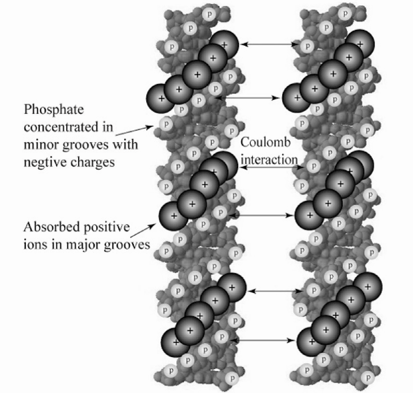
Figure 2: The pair interaction between two parallel B-DNA double helixes. The black balls with positive signs in the center represent the absorbed positive counterions, while the little grey balls represent the phosphate carrying negative charges. Each DNA duplex carries the negative charge of phosphates with area density of $16.8\mu C/cm^{2}$ plus a compensating positive charge coming from the adsorbed counterions. We take the assumption that, and the distance between them are approximately $30\textrm{\AA}$.

4.Monte Carlo Simulation
Let $t$ be the dimensionless variable to mark the time series of simulation $(t=0,1,2\ldots)$ and $T$ the environmental temperature. Assuming that $M\times N$ DNAs are on the ADNC, the position of each DNA can be represented by its coordinates $(x,y)$, where $x,y\in N$, and $0<x<M,0<y<N$. All DNA molecules in ADNC have identical sequence with $P$ base pairs. Therefore there is the collection of $M\times N\times P$ base pairs. The degree of freedom of the system is also $M\times N\times P$. The position of each base pair is thus represented by coordinates $(x,y,i)$, where $i\in N,0<i<P$. We take that the indices of base pairs is assigned from the bottom to the top of the DNA.
At the time $t_{0}$, the state for an arbitrary base pair at $(x_{0},y_{0},i)$ with well-formed hydrogen bonds is represented as $(x_{0},y_{0},i,t_{0})=1$. Contrarily, the state of a base pair with decoupled hydrogen bonds is denoted as $(x_{0},y_{0},i,t_{0})=0$ [10, 19]. $\psi(x,y,i,t)$ is a function of the time and the position of the base pair. Therefore, the state of each DNA molecules in ADNC can be represented by a sequence of digits. The number of all possible states is $2^{M\times N\times P}$.

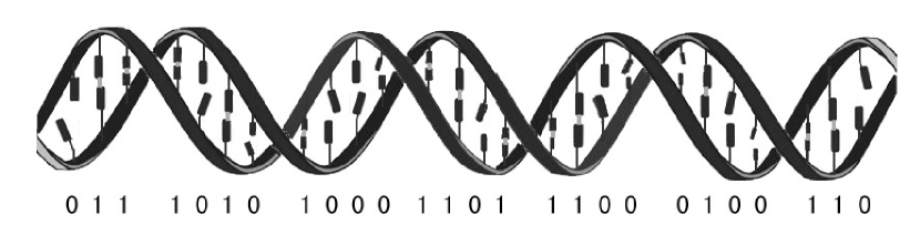
Figure 3: A schematic graph for a double-stranded DNA molecule associated with bool quantities to represent well-formed hydrogen bonds (denoted as $1$) and decoupled bonds (denoted as $0$).

The simulation begins at $t=0$, $T=0^{\,\circ}\textrm{C}$. At each step, $t$ increases by $1$, and state of base pair at $(x_{0},y_{0},i)$ is inverted, i.e. $\psi(x_{0},y_{0},i,t+1)=1-(x_{0},y_{0},i,t)$. We assume that by changing the state of the system for $M\times N\times P\times Z$ times, the system will approximate the equilibrium state infinitely. The change will be applied to each base pair for average $Z$ times. $Z$ is determined by experience and should be reasonable. We increase $T$ by $\Delta T$ during the simulation. Therefore we have the relation $T=\frac{t}{M\times N\times P\times Z}\Delta T$.
Whether the state inversion is permitted depends on the energy change ($\Delta E_{t}$) in each step. The possibility of the state change at each step is

$$P(\psi(t)\rightarrow\psi(t+1))=\left\{\begin{array}[]{c c c}1&for&\Delta E_{t}\leq 0\\ &&\\ e^{-\Delta E_{t}/k_{B}T}&for&\Delta E_{t}>0\\ \end{array}\right.$$ (6)

If the current state change is permitted, we keep up changing the system state at $t+1$. If the state change is forbidden by the possibility, the system state remains unchanged at $t$ and waits for another change at $t+1$.
To achieve a relatively precise simulation, the change of the total energy at time $t+1$ relative to that at the time $t$ is analyzed by five components. The recursion relation of energy change in each step is written as:

$$\Delta E_{t}=E(t+1)-E(t)=\sum_{l=1}^{5}\Delta E_{l}$$ (7)

where E(t+1) and E(t) are the system energy for the instant $t+1$ and $t$ respectively, and $\Delta E_{l}\,(l=1,2,3,4,5)$ is the variation of the $l$th component.
The energy change depends on both the recursion relation of the base pair at $(x_{0},y_{0},i)$ and the states of its nearest neighbors. The global energy variation is determined by the local states around the base pair $(x_{0},y_{0},i)$. Following analysis presents the recursion relation of energy changes.

4.1. The hydrogen-binding energy ($\Delta E_{1}$)
This component of the energy consists of the Morse potential (equation (3)) and kinetic energy along the orientation of the hydrogen bonds. The binding energy is independent of the states of its neighboring base pairs.

$$\Delta E_{1}=\left\{\begin{array}[]{ccc}J&if&\psi(x_{0},y_{0},i,t)=0\\ &&\\ -J&if&\psi(x_{0},y_{0},i,t)=1\\ \end{array}\right.$$ (8)

where $J(J<0)$ is the binding energy for each base pair that is in ’1’ state, while the binding energy for the ’0’ state is zero to be reference.

4.2. The stacking energy ($\Delta E_{2}$)
To simplify the calculation of the stacking energy shown in equation (2), we take into account the states of base pairs at $(x_{0},y_{0},i-1,t)$ and $(x_{0},y_{0},i+1,t)$. Their states remain unchanged during the interval from $t$ to $t+1$. We employ the periodic boundary condition (PBC) listed below.

$$\begin{array}[]{c}\psi(x+M,y,i,t)=\psi(x,y,i,t)\\ \psi(x,y+N,i,t)=\psi(x,y,i,t)\\ \psi(x,y,i+P,t)=\psi(x,y,i,t)\\ \end{array}$$ (9)

Therefore $\psi(x_{0},y_{0},i-1,t)$ and $\psi(x_{0},y_{0},i+1,t)$ are both well defined. The stacking energy reflects the interaction between nearest neighboring base pairs in same DNA, and it exists only when two nearest neighbors are in ’1’ state at the same time. We use the symbol $\psi(x,y,{i_{1},i_{2},\ldots,i_{n}},t)={b_{1},b_{2},\ldots,b_{n}}$ to denote states in the same DNA for convenience, which means $(x,y,i_{1},t)=b_{1}$, $(x,y,i_{2},t)=b_{2}$ ,…, $(x,y,i_{n},t)=b_{n}$.

$$\Delta E_{2}=\left\{\begin{array}[]{ccc}0&if&\psi(x_{0},y_{0},{i-1,i,i+1},t)=\{000\}\\ 0&if&\psi(x_{0},y_{0},{i-1,i,i+1},t)=\{010\}\\ w&if&\psi(x_{0},y_{0},{i-1,i,i+1},t)=\{001\}\\ -w&if&\psi(x_{0},y_{0},{i-1,i,i+1},t)=\{011\}\\ w&if&\psi(x_{0},y_{0},{i-1,i,i+1},t)=\{100\}\\ -w&if&\psi(x_{0},y_{0},{i-1,i,i+1},t)=\{110\}\\ 2w&if&\psi(x_{0},y_{0},{i-1,i,i+1},t)=\{101\}\\ -2w&if&\psi(x_{0},y_{0},{i-1,i,i+1},t)=\{111\}\\ \end{array}\right.$$ (10)

where $w$ is the stacking energy stored in two nearest neighboring base pairs in ’1’ state.

4.3. Morse potential away from equilibrium point ($\Delta E_{3}$)
We set $\Delta E_{1}=0$ for the uncoupled hydrogen bond at base pairs. However, for a ’0’ state is next near to a ’1’ state in the same DNA strand, the distance between two base pairs is so close that the Morse potential should be taken into account. We assigned energy $E$ to every two nearest neighboring base pairs that are in different states in the same DNA.

$$\Delta E_{3}=\left\{\begin{array}[]{ccc}2E&if&\psi(x_{0},y_{0},{i-1,i,i+1},t)=\{000\}\\ -2E&if&\psi(x_{0},y_{0},{i-1,i,i+1},t)=\{010\}\\ 0&if&\psi(x_{0},y_{0},{i-1,i,i+1},t)=\{001\}\\ 0&if&\psi(x_{0},y_{0},{i-1,i,i+1},t)=\{011\}\\ 0&if&\psi(x_{0},y_{0},{i-1,i,i+1},t)=\{100\}\\ 0&if&\psi(x_{0},y_{0},{i-1,i,i+1},t)=\{110\}\\ -2E&if&\psi(x_{0},y_{0},{i-1,i,i+1},t)=\{101\}\\ 2E&if&\psi(x_{0},y_{0},{i-1,i,i+1},t)=\{111\}\\ \end{array}\right.$$ (11)

4.4. The effect of excluded volume ($\Delta E_{4}$)
The effect of excluded volume in the nature of DNA phase transition is discussed in Fisher’s work [20]. The excluded volume effect is connected to the system entropy variation. The effect is prone to separate two complementary strands in a double helix. We use $F$ to represent the energy change corresponding to this effect. One should notice $\frac{\partial F}{\partial T}<0$. We then have

$$\Delta E_{4}=\left\{\begin{array}[]{ccc}-F&if&\psi(x_{0},y_{0},{i-1,i,i+1},t)=\{000\}\\ F&if&\psi(x_{0},y_{0},{i-1,i,i+1},t)=\{010\}\\ -F&if&\psi(x_{0},y_{0},{i-1,i,i+1},t)=\{001\}\\ F&if&\psi(x_{0},y_{0},{i-1,i,i+1},t)=\{011\}\\ -F&if&\psi(x_{0},y_{0},{i-1,i,i+1},t)=\{100\}\\ F&if&\psi(x_{0},y_{0},{i-1,i,i+1},t)=\{110\}\\ -F&if&\psi(x_{0},y_{0},{i-1,i,i+1},t)=\{101\}\\ F&if&\psi(x_{0},y_{0},{i-1,i,i+1},t)=\{111\}\\ \end{array}\right.$$ (12)

The energy changes discussed above are summarized in the figure 4 below, which does not take into account the DNA-DNA interactions so far.

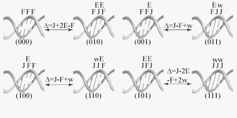
Figure 4: Scheme for the energy changes. We calculate the energy change under every case when the state of a base pair takes inversion. The value overhanging the double-arrow represents the energy variation when the state changes from left to right $\Delta=\Delta E_{1}+\Delta E_{2}+\Delta E_{3}+\Delta E_{4}$ .

4.5. DNA-DNA interaction potential ($\Delta E_{5}$)
We have introduced DNA-DNA interaction in previous section. For each base pair, we denote the state of its $m$ nearest neighbors with $\lambda_{i}$, ($i=1,2,\ldots,m;\,\lambda_{i}=0,1$). $\Delta E_{5}$ can be written as

$$\Delta E_{5}=\left\{\begin{array}[]{ccc}G\sum_{i=1}^{m}\lambda_{i}&if&\psi(x_{0},y_{0},i,t)=0\\ &&\\ -G\sum_{i=1}^{m}\lambda_{i}&if&\psi(x_{0},y_{0},i,t)=1\\ \end{array}\right.$$ (13)

where $G$ is the interaction energy between each pair of ions. Adding $\Delta E5$ to $\Delta$, we will get the energy variation including the DNA-DNA interaction.

5.Results and Discussions
Following the equation (5) - (12), we could achieve a coarse-gained simulation of the melting curves of ADNC as well as that of DNA in bulk solutions. To perform the task, we choose suitable scale parameters to carry out the simulation: $M=100$, $N=100$, $P=20$. The values of $M$ and $N$ chosen are much smaller than ones of the actual situation, which is up to $10^{4}$ in the experiment. Since we take the periodic boundary condition, the values of $M$ and $N$ used do not change our result. The starting temperature is $0\,^{\circ}\textrm{C}$, and the final temperature is $100\,^{\circ}\textrm{C}$, with increment of $0.01\,^{\circ}\textrm{C}$ for each step. To guarantee the system reaches equilibrium state, we take state changes under a specific temperature. Each base pair has average $5$ times to be changed. At each step, we count the number of DNAs that is still hybridized and calculate the percentage for dsDNA in ADNC. The simulation result shown in figure $5$ shows a steep melting transition (hollow circles), consistent to the experimental observations. The simulated result without considering DNA-DNA interaction show in filled circles in figure $5$ also agrees with the DNA melting curves in bulk solution. Comparison between the two cases suggests that the DNA-DNA interaction greatly increases the melting point of dsDNA chains.

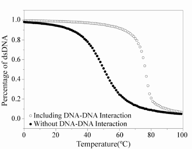
Figure 5: Simulation results of melting curves for collective DNA molecules. The filled circle represents the phase transition curve without considering the DNA-DNA interaction, while the hollow circle is the counterpart that takes into account the interaction. Parameters used in the simulations are: $J=-1900k_{B}$, $w=-250k_{B}$, $E=850k_{B}$, $F=-1650k_{B}$, $\frac{\partial F}{\partial T}=-10k_{B}$, $G=-125k_{B}$.

In conclusion, we have established a simple coarse-gained model to simulate the melting transition of DNA in ADNC. The result provides a reasonable explanation for our experimental observations. Although the simulation method discretizes the Morse potential and stacking energy proposed in Peyrard-Bishop model, the result still present a comparable approximation to experimental data due to our fine treatment of energy changes during melting transition. However, this work is only the beginning of insightful theoretical investigation for the rationality of ADNC. In future work, we will establish a more precise model to employ an extensive investigation of phase transition occurring in ADNC as well as its derived DNA machines.

Acknowledgements
This work was partly supported by the grants from Chinese Natural Science Foundation, Ministry of Science and Technology of China and financial support from Peking University.

Reference
$[1]$   Lifson S 1964 J. Chem. Phys. 40 3705
$[2]$   Poland D and Scheraga H A 1966 J. Chem. Phys. 45 1456
$[3]$   Poland D and Scheraga A H 1966 J. Chem. Phys. 45 1464.
$[4]$   Zhang Y L, Zheng W M, Liu J X, and Chen Y Z 1997 Phys. Rev. E
 56 7100
$[5]$   Theodorakopoulos N, Dauxois T and Peyard M 2000 Phys. Rev. Lett.
 85 6
$[6]$   Dauxois T and Peyard M 1995 Phys. Rev. E 51 4027
$[7]$   Dauxois T and Peyard M 1993 Phys. Rev. E 47 R44
$[8]$   Mao Y D, Luo C X, Deng W, Jin G. Y, Yu X M, Zhang Z H, Ouyang
 Q, Chen R S and Yu D P 2004 Nucleic Acids Res. 32 e144
$[9]$   Mao Y D, Luo C X and Ouyang Q 2003 Nucleic Acids Res. 31 e108
$[10]$ Zimm B H and Bragg J K 1959 J. Chem. Phys. 28 1246
$[11]$ Chrisey L A, Lee G U and O’Ferrall C E 1996 Nucleic Acids Res. 24
 3031
$[12]$ Bard A J and Fulkner L R 1980 Electrochemical methods Wiley, New
 York
$[13]$ Harreis H M, Kornyshev A A, Likos C N, Lowen H, and Sutmann G
 2002 Phys. Rev. Lett. 89 018303
$[14]$ Harreis H M, Likos C N, and Lowen H 2003 Biophys. J. 84 3607
$[15]$ Kornyshev A A and Leikin S 1997 J. Chem. Phys. 107 3656
$[16]$ Kornyshev A A 2000 Phys. Rev. E 62 2576
$[17]$ Allahyarov E and Lowen H 2000 Phys. Rev. E 62 5542
$[18]$ Kornyshev A A 2001 Phys. Rev. Lett. 86 3666
$[19]$ Hill T L 1959 J. Chem. Phys. 30 383
$[20]$ Fisher M E 1966 J. Chem. Phys. 45 1469