Chaotic desynchronization of multi-strain diseases

Abstract

Multi-strain diseases are diseases that consist of several strains, or serotypes. The serotypes may interact by antibody-dependent enhancement (ADE), in which infection with a single serotype is asymptomatic, but infection with a second serotype leads to serious illness accompanied by greater infectivity. It has been observed from serotype data of dengue hemorrhagic fever that outbreaks of the four serotypes occur asynchronously. Both autonomous and seasonally driven outbreaks were studied in a model containing ADE. For sufficiently small ADE, the number of infectives of each serotype synchronizes, with outbreaks occurring in phase. When the ADE increases past a threshold, the system becomes chaotic, and infectives of each serotype desynchronize. However, certain groupings of the primary and secondary infectives remain synchronized even in the chaotic regime.

Recently there has been a wide range of work on chaotic synchronization in dynamical systems manrubia ; pikovsky . When synchronizing chaotic systems, almost all of the work deals with coupled or connected systems BoccalettiKOVZ02 and analyzing their stability. In biological systems, such as population models, synchronization may result from coupling strengths being enhanced LloydJ04 , while desynchronization may take place as a result of vaccine control as in measles RohaniEG99 . In this work, we consider the dynamics of a single population to shed light on the phase dynamics of multi-strain diseases BartleyDG02 . The dynamics observed exhibits phase-locked regular behavior, as well as chaotic phase desynchronization between strains. Although we consider a single population model, we use the term “synchronization” to describe phase locking between variables footnote:cm .

Many population models in the past have considered single strain diseases, as in childhood diseases. In this case, the population may be grouped into the following compartments: susceptibles, infectives, and recovered Anderson91 . With no seasonal forcing included in the model, the only endemic solution to the single strain SIR models is an equilibrium point schwartz83 .

However, many diseases have co-circulating strains, or serotypes, such as influenza AndreasenLL97 , malaria GuptaTAD94 , and dengue virus FergusonDA99 . Such diseases display anti-genic diversity, exhibiting distinct serotypes when measured. Recent efforts at modeling multi-strain diseases have explored the oscillatory dynamics generated by multiple co-existing serotypes with partial cross-immunity Gog02 ; AndreasenLL97 ; EstevaV03 . However, current thinking regarding the interacting serotypes of dengue virus is that cross-reactive antibodies act to enhance the infectiousness of a subsequent infection by another serotype Vaughn00 . This is known as antibody-dependent enhancement.

It has been shown through recent serology measurements in Thailand that dengue fever, which has four co-circulating serotypes, exhibits asynchronous outbreaks. That is, each serotype has peaks that occur at different times NisalakENKTSBHIV03 . (See Fig. 7 in the Appendix.) Note that most observed infections are secondary NisalakENKTSBHIV03 , due to increased symptom severity.

In this paper, we analyze how the antibody-dependent enhancement (ADE) factor controls the onset of oscillatory outbreaks, as well as how asynchronous secondary infections are controlled dynamically.

I Description of model

To model the spread of multi-strain diseases, we follow the approach of Ferguson et. al FergusonAG99 , where they restrict the model to two serotypes. Our modeling approach differs in the general number of serotypes and in that all compartments are distinct from one another. The full model for $n$ serotypes is described below. Our simulations will be based on four serotypes, based on measured dengue data in Thailand NisalakENKTSBHIV03 .

The variable definitions are as follows: $s$, Susceptible to all serotypes; $x_{i}$, Primary infectious with serotype $i$; $r_{i}$, Primary recovered from serotype $i$; $x_{ij}$, Secondary infectious, currently infected with serotype $j$, but previously had $i$ $(i\neq j)$. The model is a system of ODEs describing the rates of change of the population fractions within each compartment cummingsthesis :

$$\frac{ds}{dt} = \mu-\beta s\sum_{i=1}^{n}\left(x_{i}+\phi\sum_{j\neq i}x_{ji}\right)-\mu_{d}s$$ (1)

$$\frac{dx_{i}}{dt} = \beta s\left(x_{i}+\phi\sum_{j\neq i}x_{ji}\right)-\sigma x_{i}-\mu_{d}x_{i}$$ (2)

$$\frac{dr_{i}}{dt} = \sigma x_{i}-\beta r_{i}\sum_{j\neq i}\left(x_{j}+\phi\sum_{k\neq j}x_{kj}\right)-\mu_{d}r_{i}$$ (3)

$$\frac{dx_{ij}}{dt} = \beta r_{i}\left(x_{j}+\phi\sum_{k\neq j}x_{kj}\right)-\sigma x_{ij}-\mu_{d}x_{ij}.$$ (4)

The parameters $\mu$, $\mu_{d}$, $\beta$, and $\sigma$ denote birth, death, contact, and recovery rates, respectively. We assume that individuals who have recovered from two infections are immune to further infection since tertiary infections are reported very rarely NisalakENKTSBHIV03 . The fixed parameters throughout the paper are given by: $\mu=\mu_{d}=0.02$, $\beta=200$, and $\sigma=100$, all with units of $years^{-1}$ cummingsthesis . (Mortality rate, $\mu_{d}$, is set equal to the birth rate so that the population remains constant in time.) Antibody-dependent enhancement is governed by the parameter $\phi$, which has not previously been measured for populations. Notice that in Eqs. 1-4, ADE enters in a nonlinear enhancement factor when $\phi>1$. We use a single $\phi$ for all strains for ease of analysis. Thus any loss of synchrony between the strains will result not from asymmetry but from the dynamics itself. Finally, notice that since the value of $\mu$ is small compared to $\beta$ and $\sigma$, it can be considered as a small parameter.

II Results

II.1 Bifurcation structure

Unlike the usual SIR models for single strains, which in the absence of forcing have only steady state behavior, the addition of multiple serotypes can induce regular and chaotic outbreaks. In particular, for a critical value of $\phi$, there exists a Hopf bifurcation to periodic oscillations. See the bifurcation diagram given in Fig. 1 for the transition from steady state to oscillatory behavior as a function of $\phi$. The usual trivial steady state, which has the population consisting of all susceptibles $(s=1)$ and the rest of the components at zero, is unstable. (The trivial solution of Eqs. 1-4 with $n=4$ serotypes has 4 unstable, 12 strongly attracting, and 5 weakly attracting directions.) The non-trivial, or endemic, steady state may be computed numerically for arbitrary $\phi$. At steady state, we notice the following: 1. The primary infectives are equal. 2. The recovered variables are equal. 3. All secondary infectives are equal.

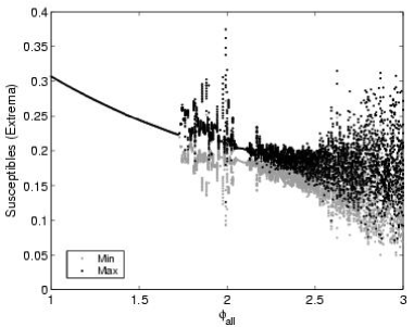
Figure 1: Bifurcation diagram for the autonomous model with $\beta=200$, $\sigma=100$, $\mu=0.02$. Shown for each $\phi$ are the maxima (black) and minima (gray) of the susceptibles during a 100 year run, after transients were removed.

Compartmental equality at steady state holds before the Hopf bifurcation point as well as after the Hopf point (although past the Hopf bifurcation point the steady state solution is unstable). We make these assumptions about the model at equilibrium, and the resulting local dynamics can be reduced to a four-dimensional system:

$$\frac{dy_{1}}{dt} = \mu-n\,\beta\,y_{1}y_{2}-n\,(n-1)\,\beta\,\phi\,y_{1}y_{4}$$ (5)

$$\frac{dy_{2}}{dt} = \beta\,y_{1}y_{2}+(n-1)\,\beta\,\phi\,y_{1}y_{4}-\sigma\,y_{2}$$ (6)

$$\frac{dy_{3}}{dt} = \sigma\,y_{2}-(n-1)\,\beta\,y_{3}y_{2}-(n-1)^{2}\,\beta\,\phi\,y_{3}y_{4}$$ (7)

$$\frac{dy_{4}}{dt} = \beta\,y_{3}y_{2}+(n-1)\,\beta\,\phi\,y_{3}y_{4}-\sigma\,y_{4}$$ (8)

Notice that for simplicity we have removed the mortality terms in each of the variables, since they are of $\mathcal{O}(\mu)$ and have a negligible effect on the steady states. Moreover, removing the mortality terms allows an analytical estimate of the endemic steady states and stability. Mortality does need to be included in the long time asymptotic runs, which we do below. The reduced model has the following steady state solution:

$$\left[\frac{\sigma}{\beta\,\left(\phi+1\right)},\frac{\mu}{n\,\sigma},\frac{\sigma}{(n-1)\,\beta\,\left(\phi+1\right)},\frac{\mu}{n\,(n-1)\,\sigma}\right].$$ (9)

Given the steady state solution as a function of $\phi$ in Eq. 9, to compute the stability we need to evaluate the linearization about the steady state. Therefore, we take the Jacobian of the vector field of the reduced model about the steady state and examine the characteristic polynomial for the eigenvalues. Recalling that $\mu$ is a small parameter, we can expand the solutions to the characteristic equation in terms of $\mu$. Since the data in NisalakENKTSBHIV03 displays four serotypes, the number of serotypes is set to $n=4$. We have a strongly attracting direction given by $z_{1}(\mu)=-\sigma+O(\mu)$, a weakly attracting direction given by $z_{2}(\mu)=-(3\,\beta\,\mu\,(\phi+1)^{2})/(4\,\sigma)+O(\mu^{2})$, and a pair of complex eigenvalues:

$$z_{\pm}(\mu)={\frac{\beta\,D(\phi)}{8\,\sigma}}\mu\,\pm\,i(\beta\mu)^{3/2}(1-f(\phi))+\mathcal{O}(\mu^{2}),$$ (10)

where $f\prime(\phi)<0$. The sign of the expression $D(\phi)\equiv 3\,{\phi}^{2}-4\,\phi-4$ determines the stability of the complex pair. Since $\phi$ is assumed to be greater than or equal to unity, $D(\phi)<0$ if $\phi\in[1,2)$ and positive otherwise. Therefore, the steady state undergoes a Hopf bifurcation at $\phi=2$. The results are close to numerical simulation, since mortality terms were dropped in the analysis but included in the simulations.

Since the reduced model does not capture the asynchronous behavior past the Hopf point, we continue our analysis using the full model. As we increase $\phi$ beyond the Hopf point, the dynamics exhibits periodic time series, as plotted in Fig. 2(a). The susceptibles exhibit a period of approximately five years when $\phi=1.725$. The actual range of stable periodic solution is quite small, and occurs over a $\Delta\phi$ of 0.004838. (See the quick transition to irregular oscillations after the steady state in the bifurcation diagram given in Fig. 1.) Past the $\phi$ value where periodic solutions become unstable, we find chaotic behavior, indicated by a positive maximum Lyapunov exponent for most $\phi$ values in that region. (The chaotic attractors persist over many initial conditions chosen from a random distribution.) We note that in this complicated region, there are small windows with attracting limit cycles resulting in a zero maximum Lyapunov exponent. Lyapunov exponents were computed by integrating linear variational equations along solutions to Eqs. 1-4. We show examples of chaotic oscillations in Fig. 2 (b) and (c) for short and long time series. Notice that in Fig. 2(c), the time series exhibits oscillatory regions which have a slowly growing envelope, interspersed with chaotic intervals. We will exploit this structure to examine how each serotype behaves dynamically.

(a)

(b)

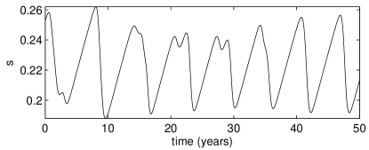
(c)

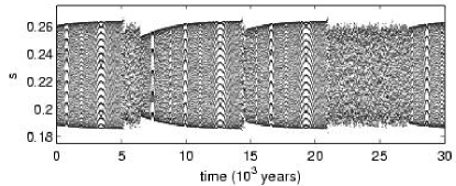
Figure 2: Time series plots of the susceptibles for the autonomous case, where $\beta=200$, $\sigma=100$, $\mu=0.02$. (a) Periodic case for ADE factor $\phi=1.725$. (b) Chaotic case for $\phi=1.73$. (c) Longer time series for chaotic case, $\phi=1.73$, with sampling once a year.

II.2 Phase analysis

Since the measured data for dengue fever shows that the serotypes oscillate out of phase, we investigate the phase of primary and secondary infectives with respect to a particular secondary infective in the full model of Eqs. 1-4. To measure phase differences with respect to a reference infective, let $Y(t)$ denote the reference infective, and $Z(t)$ another infective. Let $\{t_{k}\}$ denote the sequence of times for local maxima of $Y(t)$, and $\{\tau_{k}$} the times for local maxima of $Z(t)$. For $\tau_{m}\in(t_{k},t_{k+1})$, define the phase of $Z$ relative to $Y$ in the interval as $\Psi_{ZY}(\tau_{m})=2\pi\frac{\tau_{m}-t_{k}}{t_{k+1}-t_{k}}$.

(a)
(b)
(c)

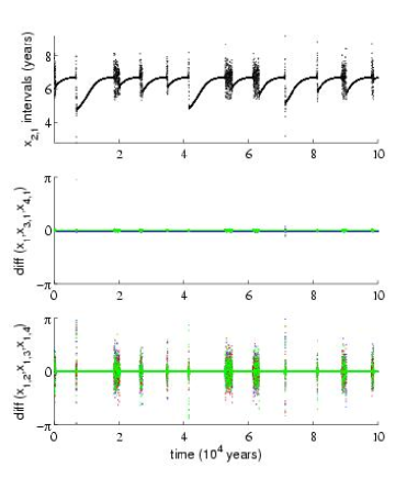
Figure 3: Phase difference analysis of time series in a chaotic region with $\phi=1.73$ for autonomous system. (a) Time intervals between local maxima of secondary infective group $x_{2,1}$. (b) Phase differences between compartments currently infected with serotype 1. Primary infective $x_{1}$ and secondary infectives $x_{3,1}$ and $x_{4,1}$ are compared to $x_{2,1}$. Maxima occur in phase. (c) Comparison between compartments currently infected with different serotypes. Secondary infectives $x_{1,2}$, $x_{1,3}$, and $x_{1,4}$ are compared to $x_{2,1}$. Maxima occur out of phase during chaotic intervals.

In Fig. 3, we compare the relative phases of infective groups for $\phi=1.73$. For the secondary infective group $x_{2,1}$, we plot the inter-maximum intervals in years in Fig. 3(a). Notice that during the non-chaotic times, the oscillation intervals grow slowly, until they begin to vary in an irregular manner during the chaotic phase. In panels (b) and (c), a direct comparison between $x_{2,1}$ and the other groups is plotted using the phase differencing equation $\Psi_{ZY}(\tau_{m})$, normalized between $-\pi$ and $\pi$. In panel (b), all other infectives who have serotype 1 as the current infection are practically in-phase with group $x_{2,1}$. In contrast, in panel (c), all those having serotype 1 as the primary infection, and currently a different serotype as the secondary infection, lose synchronization when the dynamics exhibits chaotic behavior. During the slow buildup phase, however, the groups are still synchronized. Similar desynchronization during chaotic time series occurs for the other primary and secondary infectives (not pictured here).

(a)

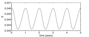
(b)                                       (c)

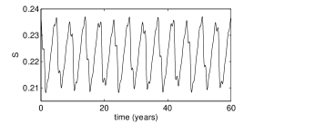
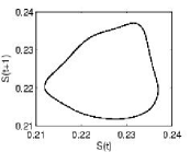
Figure 4: Dynamics of seasonally driven ADE model, where $\beta_{0}=200$, $\sigma=100$, $\mu=0.02$, and the forcing amplitude $\beta_{1}=0.05$. (a) Periodic time series of susceptible population, for the ADE factor $\phi=$1.5. (b) Quasi-periodic time series of susceptibles, for $\phi=1.7244$. (c) Projected time series sampled at intervals of one year for the susceptible population, showing the quasi-periodicity (same parameters as in (b)).

II.3 Seasonally driven case

Although the analysis suggests that chaos is responsible for the observed lag between serotypes, one could argue that since there is a seasonal component to the disease, adding a periodic forcing term should synchronize the serotypes, even when they are chaotic. To address this issue, we modified the model to include a contact rate that modulates with a period of one year; i.e., $\beta(t)=\beta_{0}(1+\beta_{1}\cos(2\pi t))$, where $\beta_{1}$ is the forcing amplitude. ($\beta_{1}=0.05$ was used in this study, but similar behavior is observed for other forcing amplitudes.) The contact rate prefactor, $\beta_{0}=200$, is constant as before. Analogous to the Hopf bifurcation in the autonomous system, bifurcation onto a torus occurs at $\phi_{c}=1.7243$. For an ADE factor below $\phi_{c}$, we observe periodic behavior, as shown in Fig. 4(a), while for an ADE factor just above $\phi_{c}$, we find quasi-periodic behavior, plotted in Figs. 4(b) and (c). In panel (c), the time series of susceptibles was sampled at the forcing period and plotted as successive iterates to show a cross-section of the torus. In both periodic and quasi-periodic cases, the serotypes are all in phase, and there is no desynchronization. However, for higher ADE, we find that the driven system becomes chaotic, and there is desynchronization.

(a)
(b)

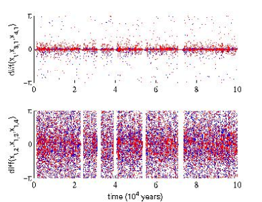
Figure 5: Chaotic phase desynchronization in periodically driven system. The ADE factor is $\phi=1.74$. (a) Phase differences between compartments currently infected with serotype 1. Primary infective $x_{1}$ and secondary infectives $x_{3,1}$ and $x_{4,1}$ are compared to $x_{2,1}$. Maxima usually occur in phase. (b) Comparison between compartments currently infected with different serotypes. Secondary infectives $x_{1,2}$, $x_{1,3}$, and $x_{1,4}$ are compared to $x_{2,1}$. Maxima occur out of phase. (Windows of synchrony occur during the oscillatory regions that have a slowly growing envelope.)

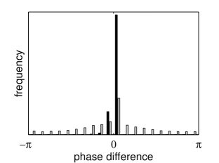
Figure 6: A histogram plot showing the statistics of the phase differences between secondary infections and primary infections from Fig. 5. Black bars: frequency of phase differences for compartments currently infected with serotype 1 (data from Fig. 5(a)), gray bars: frequency of phase differences for compartments currently infected with different serotypes (data from Fig. 5(b)).

Figure 5 shows the phase differences between the $x_{2,1}$ secondary infective and other infectives, for an ADE factor of $\phi=1.74$ and forcing amplitude $\beta_{1}=0.05$, where the solution is chaotic. Notice that in the top panel, where the phase differences are for other compartments currently infected with serotype 1, there is phase synchrony on average when compared to the case where the secondary infections are from a different serotype (second panel). Although the phase synchrony is not as good as in the autonomous case in Fig. 3, we can get a statistical measure showing how on average the phase locking compares by computing a histogram of both cases. This is shown in Fig. 6, where the grey bars correspond to phase differences of Fig. 5(b), and the black bars correspond to the data from 5(a). Notice that when comparing primary infections of serotype 1 to secondary infections that currently have serotype 1, there is a strong phase locking component on average.

III Conclusions

We have derived and analyzed the dynamics of a model for multi-strain diseases with antibody-dependent enhancement. The model for secondary infections, which includes ADE as a parameter, adds a new wrinkle to models of the SIR type. In previous studies of single strain models that do not include environmental forcing, the endemic equilibrium is the only possible stable state. That is, there are no bifurcations which give rise to dynamics exhibiting regular or irregular outbreaks. In contrast, by modeling the effect of ADE as an increase in infectivity of secondary infections, we see both analytically and numerically that periodic outbreaks appear at a critical ADE value. Moreover, the analysis reveals exactly how the period of oscillations depends on the ADE parameter near the bifurcation point. The range of periods predicted for the parameters used in our computations appear to agree well with those observed in the data in Fig. 7 in the appendix.

When the ADE factor increases above a threshold, the system’s behavior is chaotic, and outbreaks of different strains occur asynchronously. This observation corresponds qualitatively with epidemiological data on asynchronous outbreaks of dengue fever (see Appendix). Seasonal forcing, thought to be a primary driver for the observed oscillations in the different strains, is typically believed to disrupt any out-of-phase behavior in the dynamics and force the entire system to lock on the period of the forcing. However, in our preliminary study, we find that this is not the case. Phase desynchronization between serotypes occurs even in the seasonally forced case.

However, there exists a specific relationship between the primary and secondary infections. Specifically, we have observed that although the different serotypes desynchronize when the solutions are chaotic, there is surprising structure in the peak outbreaks of the serotypes when comparing the appropriate secondary infectives to the appropriate primary infectives. Although there is no vaccine currently available for all serotypes, the results here point to potential new methods of analysis and monitoring of multi-strain diseases. In the field, the majority of the cases reported are secondary infections. Therefore, by observing a small percentage of the incidence in the secondary infections of one serotype, synchronization would imply that the data is representative of the general behavior of all the groups infected with that serotype, including those with only a primary infection. Further global analysis techniques based on center manifold methods can be used to explain the synchronization of particular primary and secondary infectives when the time series becomes chaotic; this approach is the subject of further study.

Research was supported by the Office of Naval Research and the Center for Army Analysis. LB and MM were supported by the National Science Foundation under Grants DMS-0414087 and CTS-0319555. LBS is currently a National Research Council post doctoral fellow. DATC and DSB were supported by the National Institutes of Health under Grant U01GM070708 and by the National Oceanic and Atmospheric Administration under Grant NA04OAR4310138.

Appendix A Epidemiological data

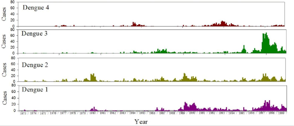
Figure 7: Frequency of detection of each of the four Dengue virus types per month at the Queen Sirikit National Institute for Child Health from 1973-1999. Reprinted from NisalakENKTSBHIV03 .

Fig. 7, reprinted from NisalakENKTSBHIV03 , shows the frequency of detection of each of the four dengue types at one hospital in Bangkok, Thailand, over a continuous 27 year period of monitoring. Infecting serotypes were defined by isolation of replication- competent virus and/or detection of viral genome in peripheral blood. (It should be noted that serological measurements were performed for only a fraction of all dengue cases.) Observe that peaks of the dengue virus types are asynchronous.

References

- (1) D. H. Z. S. C. Marubia, A. S. Mikhailov, Emergence of dynamical order (World Scientific, Singapore, 2004).
- (2) A. Pikovsky, M. Rosenblum, and J. Kurths, Synchronization: A universal concept in nonlinear science (Cambridge University Press, Cambridge, 2001).
- (3) S. Boccaletti et al., Phys. Lett. 366, 1 (2002).
- (4) A. L. Lloyd and V. A. A. Jansen, Math. Biosciences 188, 1 (2004).
- (5) P. Rohani, D. J. D. Earn, and B. T. Grenfell, Science 286, 968 (1999).
- (6) L. M. Bartley, C. A. Donnelly, and G. P. Garnett, Am. J. Trop. Med. Hyg. 96, 387 (2002).
- (7) Although it has been common practice to examine chaotic synchronization in coupled systems, it is not the most general setting. One can indeed have general slaved behavior, including chaotic saddles, in a single dynamical system, where the dynamics is constrained to a center manifold. The result is that part of the system is slaved to another. See morgan2003 for a description and review of dynamics on center and singular manifolds, and the references within.
- (8) R. Anderson and R. May, Infectious diseases of humans: Dynamics and Control (Oxford University Press, Oxford, 1991).
- (9) I. B. Schwartz, and H. L. Smith, J. Math. Bio. 18, 223 (1983).
- (10) V. Andreasen, J. Lin, and S. A. Levin, J. Math. Bio. 35, 825 (1997).
- (11) S. Gupta, K. Trenholme, R. M. Anderson, and K. P. Day, Science 263, 961 (1994).
- (12) N. M. Ferguson, C. A. Donnelly, and R. M. Anderson, Phil. Trans. R. Soc. London, Ser. B 354, 757 (1999).
- (13) J. Dawes and J. Gog, J. Math. Bio. 45, 471 (2002).
- (14) L. Esteva and C. Vargas, J. Math. Bio. 46, 31 (2003).
- (15) D. W. Vaughn et al., J. Infect. Diseases 181, 2 (2000).
- (16) A. Nisalak et al., Am. J. Trop. Med. Hyg. 68, 191 (2003).
- (17) N. Ferguson, R. Anderson, and S. Gupta, Proc. Natl. Acad. Sci. USA 96, 790 (1999).
- (18) D.A.T. Cummings, Doctoral Thesis, Johns Hopkins University, 2004.
- (19) D. Morgan, E. M. Bollt, and I. B. Schwartz, Phys. Rev. E 68, 056210 (2003).