Liquid interfaces in viscous straining flows: Numerical studies of the selective withdrawal transition

Abstract

This paper presents a numerical analysis of the transition from selective withdrawal to viscous entrainment. In our model problem, an interface between two immiscible layers of equal viscosity is deformed by an axisymmetric withdrawal flow, which is driven by a point sink located some distance above the interface in the upper layer. We find that steady-state hump solutions, corresponding to selective withdrawal of liquid from the upper layer, cease to exist above a threshold withdrawal flux, and that this transition corresponds to a saddle-node bifurcation for the hump solutions. Numerical results on the shape evolution of the steady-state interface are compared against previous experimental measurements. We find good agreement where the data overlap. However, the numerical results’ larger dynamic range allows us to show that the large increase in the curvature of the hump tip near transition is not consistent with an approach towards a power-law cusp shape, an interpretation previously suggested from inspection of the experimental measurements alone. Instead the large increase in the curvature at the hump tip reflects a logarithmic coupling between the overall height of the hump and the curvature at the tip of the hump.

1 Introduction

Topological transitions of a fluid interface are a key step in many important and complex physical processes. Simple examples include the formation and coalescence of droplets where local stresses typically determine the fluid flows near the transition. Here, we examine a different scenario where the topological transition in the interface shape is driven by a large-scale steady-state flow. Figure 1 depicts the experiment which inspired our numerical study. A deep layer of viscous silicone oil overlays a second, immiscible layer, comprised of a mixture of water and glycerin (Cohen & Nagel (2002)). Steady-state large-scale flows are created in the two fluid layers by withdrawing liquid through a tube placed in the upper layer and replenishing the same amount of liquid back into the upper layer at locations far away from the point of withdrawal. The rate of fluid withdrawal $\tilde{Q}$ dramatically affects the shape of the steady-state interface. When $\tilde{Q}$ is below a threshold value $\tilde{Q}_{c}$, the steady-state interface forms a hump. The lower-layer flow has the form of a toroidal recirculation, with a stagnation point at the tip of the hump. Since only liquid in the upper layer is withdrawn into the tube, this is known as the selective withdrawal regime. When the withdrawal flux $\tilde{Q}$ is larger than $\tilde{Q}_{c}$, the flows and the interface remain steady, but the interface attains a different topology. The steady-state interface is now “open” and has the shape of a spout which extends smoothly into the tube. Since liquid is now withdrawn from both layers, this is known as the viscous entrainment regime. In this regime, the amount of liquid in the lower layer slowly decreases while the amount of liquid in the upper layer slowly increases. The large-scale toroidal recirculation in the lower-layer is weakly perturbed by the onset of entrainment. The stagnation point is deflected slightly downwards, from the hump tip to the interior.

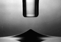
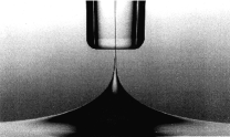
Figure 1: (a) Schematic of experiment. Liquid is withdrawn at a prescribed volume flux $\tilde{Q}$ through a tube inserted into the top layer and replenished at the same rate. The top layer is a viscous silicone oil. The bottom layer is a mixture of water and glycerin. The two layers have comparable viscosities. The flow rates are small so that viscous effects are significant in both layers. The tube diameter is 1.6 mm. (b) Selective withdrawal regime: below $\tilde{Q}_{c}$ a steady-state hump forms on the interface. (c) Viscous entrainment regime: above $\tilde{Q}_{c}$ a steady-state spout forms. Photos courtesy of Cohen & Nagel.

 

Analogous transitions from selective withdrawal to entrainment occur in many industrial and physical processes. Some examples on large lengthscales include the intrusion of water into an oil reservoir during the last stages of petroleum recovery (Renardy & Joseph (1985); Renardy & Renardy (1985)), water-coning in sandy beds (Forbes et al. (2004)), the formation of long-lived plumes by thermal convection in the earth’s mantle (Jellinek & Manga (2002)) and pollution recovery on lakes and oceans (Imberger & Hamblin (1982)). On small lengthscales, the bursting of a liquid drop in a steady straining flow (Taylor (1934); Grace (1982); Rallison & Acrivos (1978); Stone (1994)), the deposition of a thin trailing tendril by a drop sliding down an incline (Limat & Stone (2004)) and the formation of thin cylindrical tendrils and droplets in microfluidic devices using axisymmetric flow-focusing (Anna et al. (2003); Link et al. (2004); Lorenceau et al. (2005); Utada et al. (2005)) all involve topological transition of steay-state interfaces.

In the selective withdrawal experiments, the curvature at the hump tip increases significantly as the transition is approached from below Cohen & Nagel (2002); Cohen (2004). Intriguingly, measurements of the hump height and curvature evolution near the transition suggest the steady-state hump shape evolves towards a power-law cusp. In order to explain this apparent divergence, Cohen and Nagel made an analogy to recent works on topological transitions that correspond to the formation of a finite-time singularity in the governing equations. Some examples are the break-up of a liquid drop into two daughter drops (Eggers (1997); Cohen et al. (1999); Zhang & Lister (1999); Doshi et al. (2003)), the coalescence of two drops into one (Oguz & Prosperetti (1990); Eggers et al. (1999); Thoroddsen et al. (2005)), and the eruption of an electrohydrodynamic spout under the sudden application of a large electric-field (Oddershede & Nagel (2000)). In all these situations, the topology change necessarily requires a divergence in the mean curvature at a point on the interface. As a result, the Laplace pressure due to surface tension, which is proportional to the mean curvature, diverges as well, thereby creating a singularity in the governing equations. This suggested analogy between the topological transition in viscous withdrawal and finite-time singularity formation is surprising. While the break-up of a liquid drop requires that the interface deforms continuously from a single, connected shape to several disconnected shapes, and therefore requires the formation of a singular shape at break-up, the topological transition in this experiment deals with changes in the steady-state interface shape. Therefore the transition from selective withdrawal to viscous entrainment does not require that the hump shape evolve into the spout shape continuously as a function of the withdrawal flux $\tilde{Q}$. Generically, one would expect a discontinuous change in the steady-state shape across the selective withdrawal to viscous entrainment threshold. The apparently, nearly continous shape-change observed in the experiment is, therefore, rather unusual.

This surprise motivates our work. Here we conduct a numerical analysis of a model withdrawal process in which the interface deformation is solely controlled by viscous stresses and surface tension. We focus on the selective withdrawal regime and analyze how the interface fails at the transition. In particular we are interested in elucidating the various factors that determine the final hump shape. Experiments show that this final shape is well correlated with the minimum spout thickness attained in the viscous entrainment regime (figure 1c). Consequently, a detailed understanding of this topological transition will help advance a variety of practical applications. One such application entails takeing advantage of viscous entrainment to encapsulate biological cells for transplant therapy (Cohen et al. (2001); Wyman et al. (2004)). In this technique, the minimum spout size directly determines the minimum thickness of a protective polymer coating that can be applied to the cells.

The rest of this paper is organized as follows: In section 2 we discuss related works and background materials. In section 3 we describe the model withdrawal process and its numerical formulation for a system in which the upper and lower fluid viscosities are equal. In section 4 we analyse solutions to the model. Section 4.1 describes in detail the interface evolution near the transition and the sharpening of the hump tip. We find that scalings of the hump curvature and hump height with the rate of withdrawal identify the transition as a saddle-node bifurcation. In accordance with this picture we find that the hump solution remains smooth as the transition is approached. Surprisingly, we also find that near the transition, the hump height couples logarithmically to the curvature at the hump tip. In section 4.2, we show that, for the equal viscosity layers investigated, these key findings are independent of the particular withdrawal conditions in the numerical simulations. In section 4.3, we compare the numerical and experimental results and find excellent agreement between them. Moreover, we show that the unusual logarithmic coupling between the hump height and the hump curvature can easily lead to a misinterpretation that the system approaches a steady state singularity at the transition. A more detailed discussion of the distinction between the previous interpretation and our results is presented in section 5.

Our findings indicate the transition from selective withdrawal to viscous entrainment involves a discontinuous change in the steady-state shape that has the structure of a saddle-node bifurcation. This discontinuity is effectively obscured in practice by the logarithmic coupling between the hump height and the hump curvature, which causes changes in the hump curvature to be far larger, and therefore more evident, than changes in the hump height as the transition is approached.

2 Background

Many different realizations of flow-driven topological transitions have been investigated in previous works. Here, we review those studies that directly assess the ingredients necessary for a topological transition to take place and the appropriate ways of characterizing the evolution of the interface near such a transition.

2.1 Viscous entrainment in the absence of surface tension

A number of experimental and theoretical works have focused on the transition from selective withdrawal to viscous entrainment in stratified, two-layer systems where surface tension effects are assumed to be either negligible or weak. These studies were motivated by geophysical flows, in particular the emptying of a magma chamber during a volcanic explosion. Blake & Ivey investigated the threshold withdrawal flux $\tilde{Q}_{c}$ necessary for the onset of entrainment in miscible, stratified layers (Ivey & Blake (1985)). In a follow up numerical study (Lister (1989)), Lister analyzed the onset of entrainment in two liquid layers of equal viscosity and found that a finite value for $\tilde{Q}_{c}$ exists only if surface tension effects, however small, are included in the analysis. These studies did not analyze the hump evolution near the transition.

2.2 2-D analogues

Air entrainment, such as occcurs in high-speed coating (Simpkins & Kuck (2000)) and in the impact of a jet of viscous liquid into a layer of the same viscous liquid (Lorenceau et al. (2004)) is often accompanied by the interface approaching a two-dimensional power-law cusp shape (Joseph et al. (1991)). Jeong & Moffatt showed analytically that, in the idealized limit where air flow effects are negligible, there is no transition from selective withdrawal to air entrainment (Jeong & Moffatt (1992)). Instead the interface shape approaches a steady-state singularity in the shape of a power-law cusp as the flow rate is increased towards infinity. More recent thereotical and experimental analyses (Eggers (2001); Lorenceau et al. (2003)) showed that, when air flow effects are included, they perturb the idealized dynamics so that a transition to air entrainment occurs at finite flow rate. The approach towards a steady-state singularity is then cut-off at a small lengthscale. Since the cut-off for air entrainment originates from viscous stresses associated with air flow, the cut-off lengthscale has a strong dependence on the viscosity contrast and increases as $(\mu_{0}/\mu)^{4/3}$, where $\mu_{0}$ is the air viscosity.

2.3 Selective withdrawal in 3D with viscous flow and surface tension

In their studies of 3-D axisymetric selective withdrawal, Cohen & Nagel (Cohen & Nagel (2002)) used two liquids of comparable viscosities and measured $\tilde{h}$, the hump height, and $\tilde{\kappa}$, the mean curvature at the hump tip, as a function of the withdrawal flux $\tilde{Q}$. In a follow up study Cohen (Cohen (2004)) analyzed the transition for different pairs of liquids. In particular, the viscosity ratio, defined as the viscosity of the liquid to be entrained divided by the viscosity of the entraining liquid, was varied from $O(1)$ to $10^{-3}$. Analysis of the measurements show that, as the transition from selective withdrawal to viscous entrainment is approached from below, the steady state hump curvature increases dramatically. Cohen and Nagel showed that this rate of increase can be fit to a power law divergence. They also noted however, that the hump never reaches a cusp shape. Instead the final stage of the hump evolution is cut off by the transition. This behavior lead to the interpretation that a singular solution for the steady-state shape organizes the nearly continuous transition between the steady-state hump and spout shapes. The transition from a hump to a spout was observed to occur when the radius of curvature at the hump tip was O($50$) $\mu$m or more. Moreover, the cut-off lengthscale shows little dependence on the viscosity contrast between the two layers. Consequently axisymmetric viscous withdrawal in 3D differes strikingly from air entrainment in 2D, which shows a strong dependence of the cut-off lengthscale on the viscosity contrast.

2.4 Viscous drainage

An analogous, but not necessarily equivalent, topology change occurs in viscous drainage experiments, in which a viscous liquid exposed to air is placed in a container with an opening at the bottom surface and is allowed to drain out of the container due to its own weight (Chaieb (2004); Courrech du Pont & Eggers (2006)). As in the setup by Cohen & Nagel, the drainage creates a large-scale toroidal recirculation whose viscous stresses deform the interface. Thus the drainage experiment resemble an upside-down version of the two-layer withdrawl experiment. A key difference is that the layer depth of the withdrawn fluid changes with time in the drainage experiment, but remains constant in the setup used by Cohen & Nagel. As the liquid drains out and the layer depth decreases below a critical value, a sharp cusp develops on the interface, a feature identified by Correch du Pont & Eggers as a steady-state singularity. A further decrease in the layer depth causes the cusp to approach closer to the bottom surface and eventually intrude into the aperture through which the fluid is draining. Correch du Pont & Eggers report that there is no transition from selective withdrawal to viscous entrainment throughout the entire drainage process. Moreover, the maximum curvature obtained in the drainage experiments, which corresponds to using two fluid layers with a viscosity contrast of $10^{-6}$, are far larger than the maximum curvature measured by Cohen & Nagel for two fluid layers with a viscosity contrast of $10^{-3}$. The origin of these different outcomes is, at present, not understood.

2.5 Viscous withdrawal in 3D with surface tension

Motivated by the thin stable spout created in the viscous entrainment regime, Zhang analyzed the transition in the reverse direction, from viscous entrainment to selective withdrawal. The analysis focuses on the regime where the viscosity of the fluid entrained is far smaller than the viscosity of the entraining liquid, and constrains the spout shape to be nearly cylindrical throughout (Zhang (2004)). These simplifications allow the steady-state spout shape to be described via a long-wavelength model. Surprisingly, results for the model show that, changing the boundary conditions on the interface, without changing the material parameters, can profoundly change the nature of the shape transition. For some boundary conditions, the steady-state interface deforms continuously with withdrawal flux from a spout to a hump across the transition. For other boundary conditions, the steady-state interface changes discontinuously at the transition. Thus, there appears to be a subtle interplay between the entraining flow and surface tension effects. As a result, the transition is strongly influenced by constraints on the large-scale shape of the interface. Case & Nagel have recently characterized the steady-state spout shape experimentally (Case & Nagel (2006)).

2.6 Emulsification

Another extensively studied shape transition that has strong points of similarity with the selective withdrawal to viscous entrainment transition occurs when a single liquid drop is emulsified into several drops by an axisymmetric straining flow (Taylor (1934); Rallison & Acrivos (1978); Grace (1982); Stone (1994)). In both situations, an imposed flow far from the interface induces flows near the interface between two viscous liquids. The steady-state interface is deformed at low flow rates and “broken” at high flow rates. The crucial differences are that, for drop emulsification, there is no steady-state interface above the threshold flow rate. The drop is simply stretched out indefinitely by the flow. Also, even in the analog of the selective withdrawal regime, when a steady-state shape exists for the drop, the flow dynamics are different because the flow inside the drop must assume a form satisfying global volume conservation. In contrast, for the two-layer withdrawal experiment, the layer depth is always much larger than the hump height. It is then reasonable to expect that the global volume constraint does not introduce a significant modification to the flow dynamics. We will show this expectation is indeed borne out by results from the numerics.

The viscosity contrast between the drop and surrounding fluid strongly affects the deformation-to-burst transition. When the drop is far less viscous than the surrounding liquid, the steady-state shape approaches a cusp shape as the burst transition is approached from below. In particular, the radius of curvature at the two, elongated ends of the liquid drop is cut-off on an exponentially small lengthscale (Acrivos & Lo (1978)). Long-wavelength analyses of the extended drop shape in this regime also show that the burst transition corresponds to a saddle-node bifurcation in the leading-order solution for the overall drop shape (Taylor (1964); Buckmaster (1973)). When the drop viscosity is comparable with the surrounding liquid, the steady-state shape remains nearly spherical as the burst transition is approached. Recently, numerics and phenomenological arguments have shown that the shape transition when the drop viscosity is equal to the surrounding liquid viscosity corresponds to a saddle-node bifurcation (Navot (1999); Blawzdziewicz et al. (2002)).

2.7 Inviscid selective withdrawal

Finally, we note that a similar flow-driven topological transition exists at high Reynolds number when water drains out of a filled bathtub (Sautreaux (1901); Lubin & Springer (1967)). In practice, this is always accompanied by the formation of a vortex. More generally, withdrawal from two stratified layers of inviscid fluids is relevant for transport in water storage reservoirs, where often a layer of fresh water overlies a layer of salty water (Imberger & Hamblin (1982)). Intriguingly, some of the results for the idealized problem of withdrawal from two layers of perfectly inviscid fluids (Tuck & Vanden-Broeck (1984); Vanden-Broeck & Keller (1987); Miloh & Tyvand (1993)) suggest that, for the inviscid fluid system, the transition from selective withdrawal to full entrainment corresponds to the formation of a singular shape on the steady-state interface. This has motivated many recent theoretical and numerical studies, despite the fundamental difficulty that, without the small-scale smoothing provided by viscosity and/or surface tension in real life, the idealized problem is fundamentally ill-posed and can only be approached via careful limiting processes. For the same reason, direct comparison with experiments has also been difficult. For our study, the most relevant and suggestive results are that two-dimensional withdrawal differs significantly from axisymmetric withdrawal (Forbes et al. (2004); Stokes et al. (2005)). Also, in both 2D and axisymmetric withdrawal, whether selective withdrawal or full entrainment is realized can depend crucially on the initial conditions which determine transient evolution of the interface, instead of being solely determined by the boundary conditions (Hocking & Forbes (2001)).

In sum this review of viscous flow driven topological transitions shows studies of flow-driven topological transitions have produced a wealth of surprises. The wide range of behaviors observed indicate that apparently trivial differences in the exact experimental configurations can have a dramatic effect on the transition structure. On the other hand, the interface evolution observed in these different situations shares a number of common features, such as the existence of a topological transition at a finite flow-rate, and the development of small-scale features on the interface near the transition. In order to make progress on the 3-D selective withdrawal problem, it is likely that experiments, simulations and theoretical calculations, all of which address the same flow geometry, will be needed. This is one reason why our study focuses on devising and analyzing a model withdrawal process that can be directly compared with the previous experiments (Cohen & Nagel (2002)).

3 Modeling Selective Withdrawal

This section describes our numerical model in the following order: we first identify the key parameters in the viscous withdrawal experiments by Cohen & Nagel and then describe an idealized withdrawal problem which retains these key features. A numerical formulation of the idealized problem, together with the approximations, is given in section 3.1. Section 3.2 gives details of the numerical implementation. The key approximations are that in our calculation the gradual flattening of the liquid interface due to hydrostatic pressure on large lengthscales is approximated by a hard-cutoff lengthscale $a$. The gradual decay of the induced flow in the lower layer below the interface is approximated by a cut-off condition requiring that the pressure in the lower layer becomes uniform laterally across the liquid layer. Comparisons of results obtained using these approximations against those calculated using more realistic boundary conditions (section 4.2) and the experiment (section 4.3) show that the key features of the withdrawal are well reproduced by the simple numerical model.

In the experiment, the height of the hump created is at most a few millimeters. The tube height $S_{p}$ is comparable in size, ranging from $0.255$ cm to $0.830$ cm. The capillary lengthscale $\ell_{\gamma}$, which characterizes the relative importance of surface tension and hydrostatic pressure, is about $0.55$ cm. Deformations on lengthscales below $\ell_{\gamma}\equiv\sqrt{\gamma/\Delta\rho g}$ are stabilized by surface tension. Deformations on lengthscales above $\ell_{\gamma}$ are stabilized by hydrostatic pressure. All these lengthscales are much smaller than the dimensions of the liquid layer which is $12$ cm deep and $30$ cm in extent. Also, when tube height is sufficiently large, the interface deformation changes very little when the tube diameter is changed. This is the regime in which all the experimental data were taken.

Since the tube height $S_{p}$ and the capillary lengthscale $\ell_{\gamma}$ are comparable, both lengthscales are expected to influence the dynamics. As a result, there are several reasonable ways to define the Reynolds number, and it is unclear how the Reynolds number of the withdrawal flow should change with $S_{p}$ or $\ell_{\gamma}$. To avoid this ambiguity, we use the observed hump height $\tilde{h}$ as the characteristic lengthscale and define the Reynolds number $Re$ as $\rho\tilde{Q}\tilde{h}/(\mu 4\pi S^{2}_{p})$, where $\rho$ is the density of the upper liquid, $\mu$ the viscosity of the upper layer, and $\tilde{Q}/4\pi S^{2}_{p}$ a typical flow rate. An estimate using parameters from the experiment yields $Re\approx 0.1$, indicating that inertial effects are small. The stress balance on the interface is therefore characterized by the capillary number,

$$Ca=\frac{\mu}{\gamma}\frac{\tilde{Q}}{4\pi S^{2}_{p}}$$ (1)

a ratio of the strength of the viscous stresses exerted by the flow relative to the Laplace pressure due to surface tension. For a typical experiment, the transition from selective withdrawal to viscous entrainment corresponds to a threshold capillary number $Ca_{c}$ in the range of $10^{-3}$. Thus surface tension effects are strong even at the transition.

3.1 Minimal Model

These results from the two-layer viscous withdrawal experiment motivate the following idealization. Since the container size is much larger than the characteristic lengthscale of the hump, the two immiscible liquid layers are taken as infinite in extent and in depth. We use a cylindrical coordinate system where $z=0$ corresponds to the height of the undisturbed, flat interface and $r=0$ is the centerline of the withdrawal flow. To drive the withdrawal, we prescribe a sink flow

$$\mathbf{u}_{\textrm{ext}}(\mathbf{x})=\frac{\tilde{Q}}{4\pi|\mathbf{x}_{S}-\mathbf{x}|^{2}}(\mathbf{x}_{S}-\mathbf{x})$$ (2)

where $\mathbf{x}_{s}=\tilde{S}\mathbf{e_{z}}$ corresponds to a sink placed at height $\tilde{S}$ above the undisturbed interface and $\tilde{Q}$ is the strength of the point sink. This choice allows $\tilde{S}$ to be the only lengthscale imposed on the flow, consistent with the experimental observation that the hump shape depends primarily on the height of the withdrawal tube $S_{p}$ and not on its diameter. Instead of explicitly including the effect of hydrostatic pressure, we require that the interface is deformed by the withdrawal flow only within the region $0\leq r\leq a$. The interface $S_{I}$ is pinned at $0$ deflection at $r=a$. Beyond this point, the interface is taken to be entirely flat. Physically this hard cut-off, or pinning length $a$ corresponds roughly to the capillary lengthscale $\ell_{\gamma}$. In the calculation the slope of of the interface at $r=a$ is adjusted so that the pinning condition is satisfied at all flow rates. This introduces an error in the interface shape near $r=a$. This error is guaranteed to be small when the sink height $\tilde{S}$ is far smaller than $a$. It turns out to be also small even when $\tilde{S}$ is comparable with $a$. (In the experiment, tube height $S_{p}$ is either comparable with or smaller than the capillary lengthscale $\ell_{\gamma}$.)

Finally, since the Reynolds number associated with flows in the experiment is small and the interface evolution is observed to remain essentially the same even as the layer viscosities are made unequal, we idealize the flow dynamics in both liquids to be purely viscous. We also assume the two liquids have exactly the same viscosity. These assumptions mean that the flow dynamics in the upper layer satisfies

$$\mathbf{\nabla}\cdot\mbox{\boldmath$\sigma$}_{1}=-\mathbf{\nabla}p_{1}+\mu\mathbf{\nabla}^{2}\mathbf{u}_{1}=\mathbf{0},\quad\mathbf{\nabla}\cdot\mathbf{u}_{1}=\mathbf{0}$$ (3)

where $\mathbf{u}_{1}$ is the disturbance velocity field created in the upper layer due to the presence of the liquid interface, $p_{1}$ is the pressure and $\mbox{\boldmath$\sigma$}_{1}$ is the stress field associated with the disturbance velocity field $\mathbf{u}_{1}$. Note $\mathbf{u}_{\rm ext}$ is a solution of Laplace’s equation and therefore does not give rise to a uniform pressure distrubtion. The flow in the lower layer is created solely via the flow in the upper layer past the interface. Therefore, $\mathbf{u}_{2}$, the disturbance velocity field in the lower layer, satisfies

$$\mathbf{\nabla}\cdot\mbox{\boldmath$\sigma$}_{2}=-\mathbf{\nabla}p_{2}+\mu\mathbf{\nabla}^{2}\mathbf{u}_{2}=\mathbf{0},\quad\mathbf{\nabla}\cdot\mathbf{u}_{2}=\mathbf{0}$$ (4)

where $p_{2}$ is the pressure field in the lower layer, $\mbox{\boldmath$\sigma$}_{2}$ the fluid stress field in the lower layer.

Since the flow dynamics in both layers are completely viscous, and therefore described by the linear Stokes equations, we can represent the velocity field as an integral over a suitably defined closed surface, as discussed in earlier works and in textbooks on viscous flow (Lorentz (1907); Ladyzhenskaya (1963); Pozrikidis (1992)). As a reminder, the key result of the boundary integral formulation is that a Stokes velocity field $\mathbf{u}$ at a point $\mathbf{x}$ is given by an integral over any closed surface $S$ enclosing $\mathbf{x}$. The surface integral has the form

$$\mathbf{u}(\mathbf{x})=\int_{S}\mbox{\boldmath$J$}(\mathbf{r})\cdot[\mathbf{n}\cdot\mbox{\boldmath$\sigma$}(\mathbf{y})]\ \rm dS_{\mathbf{y}}+\int_{S}\mathbf{n}\cdot\mbox{\boldmath$K$}(\mathbf{r})\cdot\mathbf{u}(\mathbf{y})\ \rm dS_{\mathbf{y}}$$ (5)

where $\mathbf{y}$ is the point on the surface that you are integrating over and $\mathbf{n}$ is an outward-pointing surface normal. The tensors $\mathbf{J}$ and $\mathbf{K}$ are defined as:

$$\mathbf{J}(\mathbf{r})=\frac{1}{8\pi\mu}\left(\frac{\mathbf{1}}{r}+\frac{\mathbf{rr}}{r^{3}}\right)\qquad\mathbf{K}(\mathbf{r})=-\frac{3}{4\pi}\frac{\mathbf{rrr}}{r^{5}}\qquad\mathbf{r}=\mathbf{x}-\mathbf{y}.$$

Physically, equation (5) says that the velocity at the interior point $\mathbf{x}$ can be expressed as a sum over two different kinds of contributions over the the closed surface $S$. The first term on the right hand side of equation (5) corresponds to the component of fluid stress normal to the surface $S$ exerted by flows past the enclosing surface. The second contribution corresponds to flows into and along the closed surface $S$ (second term on the right hand side of equation (5)). If the point $\mathbf{x}$ lies outside the volume enclosed, then the contributions over the closed surface cancel, so that the right hand side of (5) sums to $0$. A point on the closed surface $S$ is a special case. When the closed surface $S$ is continuous and smoothly varying, the velocity at $\mathbf{x}$ is simply an average of the contribution from $S$ to $\mathbf{x}$ if it were in the exterior and the contribution from $S$ to $\mathbf{x}$ if it were an interior point. As a result, the velocity for a point $\mathbf{x}$ on the surface $S$ can be written as

$$\frac{1}{2}\mathbf{u}(\mathbf{x})=\int_{S}\mbox{\boldmath$J$}(\mathbf{r})\cdot[\mathbf{n}\cdot\mbox{\boldmath$\sigma$}(\mathbf{y})]\ \rm dS_{\mathbf{y}}+\int_{S}\mathbf{n}\cdot\mbox{\boldmath$K$}(\mathbf{r})\cdot\mathbf{u}(\mathbf{y})\ \rm dS_{\mathbf{y}}.$$ (6)

These results allow us to derive an integral equation for the time-evolution of the interface in our idealized withdrawal problem. To begin, we note that we can enclose the entire upper layer as follows: first we define the surface $S_{\infty}$, which has the shape of a hemispherical shell with radius $R_{\infty}$. As $R_{\infty}$ goes to infinity, the surface $S_{\infty}$ and the liquid interface $S_{I}$ encloses all the liquid in the upper layer. From (5), we can write the disturbance velocity $\mathbf{u}_{1}$ in the upper layer as

$$\mathbf{u}_{1}(\mathbf{x})=\int_{S_{I}+S_{\infty}}\mbox{\boldmath$J$}\cdot(\mathbf{n}\cdot\mbox{\boldmath$\sigma$}_{1})\ \rm dS_{\mathbf{y}}+\int_{S_{I}+S\infty}\mathbf{n}\cdot\mbox{\boldmath$K$}\cdot\mathbf{u}_{1}\ \rm dS_{\mathbf{y}}.$$ (7)

Since $\mathbf{u}_{1}$ decays rapidly to $\mathbf{0}$ at infinity, the contribution from the shell $S_{\infty}$ approaches $0$ as $R_{\infty}$ is taken to infinity. As a result, the only remaining contributions are due to the liquid interface $S_{I}$, so that we can write the disturbance velocity $\mathbf{u}_{1}$ in the upper layer as

$$\mathbf{u}_{1}(\mathbf{x})=\int_{S_{I}}\mbox{\boldmath$J$}\cdot(\mathbf{n}\cdot\mbox{\boldmath$\sigma$}_{1})\ \rm dS_{\mathbf{y}}+\int_{S_{I}}\mathbf{n}\cdot\mbox{\boldmath$K$}\cdot\mathbf{u}_{1}\ \rm dS_{\mathbf{y}}$$ (8)

From (6), the velocity at a point on the interface is given by

$$\frac{1}{2}\mathbf{u}(\mathbf{x})=\int_{S_{I}}\mbox{\boldmath$J$}\cdot(\mathbf{n}\cdot\mbox{\boldmath$\sigma$}_{1})\ \rm dS_{\mathbf{y}}+\int_{S_{I}}\mathbf{n}\cdot\mbox{\boldmath$K$}\cdot\mathbf{u}_{1}\ \rm dS_{\mathbf{y}}\quad\textrm{ for }\mathbf{x}\in S_{I}.$$ (9)

Finally, consider a point $\mathbf{x}$ on the surface $S_{R}$ given by $z=0$, as sketched in figure  2. At a finite withdrawal flux, the interface is deflected away from the $z=0$ plane. As a result, points on $S_{R}$ lie entirely inside the lower layer and therefore are not enclosed by the surface $S_{I}+S_{\infty}$, therefore the contribution from the surface integral over $S_{I}+S_{\infty}$ vanish at a point $\mathbf{x}$ on $S_{R}$, or

$$\mathbf{0}=\int_{S_{I}}\mbox{\boldmath$J$}\cdot(\mathbf{n}\cdot\mbox{\boldmath$\sigma$}_{1})\ \rm dS_{\mathbf{y}}+\int_{S_{I}}\mathbf{n}\cdot\mbox{\boldmath$K$}\cdot\mathbf{u}_{1}\ \rm dS_{\mathbf{y}}\quad\textrm{ for }\mathbf{x}\textrm{ in lower layer.}$$ (10)

Figure 2: Simplified numerical model of selective withdrawal. The upper and lower liquid layer is separated by an interface $S_{I}$, constrained so that the deflection is nonzero only within a radius $a$. At a finite withdrawal flux, the surface $S_{R}$ lies entirely within the lower layer.

 

Next we consider the volume of liquid in the lower layer enclosed by the closed surface comprised of $S_{R}$ and $S_{I}$. Again, starting with (6), we can write the velocity at a point $\mathbf{x}$ on either the liquid interface $S_{I}$ or the surface $S_{R}$, henceforth referred to as the “reservoir surface”, as

$$\frac{1}{2}\mathbf{u}(\mathbf{x}) = \int_{S_{I}}\mbox{\boldmath$J$}\cdot(\mathbf{n}\cdot\mbox{\boldmath$\sigma$}_{2})\ \rm dS_{\mathbf{y}}+\int_{S_{I}}\mathbf{n}\cdot\mbox{\boldmath$K$}\cdot\mathbf{u}_{2}\ \rm dS_{\mathbf{y}}+\int_{S_{R}}\mbox{\boldmath$J$}\cdot(\mathbf{n}\cdot\mbox{\boldmath$\sigma$}_{2})\ \rm dS_{\mathbf{y}}$$

$$+ \int_{S_{R}}\mathbf{n}\cdot\mbox{\boldmath$K$}\cdot\mathbf{u}_{2}\ \rm dS_{\mathbf{y}}\quad\textrm{ for }\mathbf{x}\in S_{I}\textrm{ or }S_{R}$$

where $\mathbf{n}$ again is an outward pointing surface normal. As a result, for a point $\mathbf{x}$ on the liquid interface $S_{I}$, the surface integral over $S_{I}$ in (3.1) has exactly the opposite sign as the surface integral over $S_{I}$ in (9). Since the velocity is continuous across the interface, the two surface integrals involving the $\mathbf{K}$ tensor cancel exactly when the two equations, (3.1) and (9), for the velocity at a point $\mathbf{x}$ on the interface are added together. As a result, the velocity on the liquid interface can be re-written as

$$\mathbf{u}(\mathbf{x}) = \int_{S_{I}}\mbox{\boldmath$J$}\cdot[\mathbf{n}\cdot\mbox{\boldmath$\sigma$}]_{-}^{+}\,\rm dS_{\mathbf{y}}+\int_{S_{R}}\mbox{\boldmath$J$}\cdot(\mathbf{n}\cdot\mbox{\boldmath$\sigma$}_{2})\ \rm dS_{\mathbf{y}}$$

$$+ \int_{S_{R}}\mathbf{n}\cdot\mbox{\boldmath$K$}\cdot\mathbf{u}_{2}\ \rm dS_{\mathbf{y}}\quad\textrm{ for }\mathbf{x}\in S_{I}$$

where $[\mathbf{n}\cdot\mbox{\boldmath$\sigma$}]_{-}^{+}=\mathbf{n}\cdot\mbox{\boldmath$\sigma$}_{1}-\mathbf{n}\cdot\mbox{\boldmath$\sigma$}_{2}$ denotes the jump in the normal stress across $S_{I}$ due to surface tension and is equal to $2\gamma\kappa\mathbf{n}$ where $\kappa$ is the mean surface curvature and $\mathbf{n}$ points outwards from $S_{I}$ and $S_{R}$. Similarly, adding (10) and (3.1) yields an expression for the velocity at a point $\mathbf{x}$ on the reservoir surface $S_{R}$

$$\frac{1}{2}\mathbf{u}_{2}(\mathbf{x}) = \int_{S_{I}}\mbox{\boldmath$J$}\cdot[\mathbf{n}\cdot\mbox{\boldmath$\sigma$}]_{-}^{+}\,\rm dS_{\mathbf{y}}$$

$$+\int_{S_{R}}\mbox{\boldmath$J$}\cdot(\mathbf{n}\cdot\mbox{\boldmath$\sigma$}_{2})\ \rm dS_{\mathbf{y}}+\int_{S_{R}}\mathbf{n}\cdot\mbox{\boldmath$K$}\cdot\mathbf{u}_{2}\ \rm dS_{\mathbf{y}}\quad\textrm{ for }\mathbf{x}\in S_{R}.$$

Equations (3.1) and (3.1) together provide an expression for the velocity on the liquid interface as a function of the interface shape, and $\mathbf{n}\cdot\mbox{\boldmath$\sigma$}|_{S_{R}}$, the normal stress exerted by flow in the lower layer on the reservoir surface $S_{R}$. In a full calculation, $\mathbf{n}\cdot\mbox{\boldmath$\sigma$}|_{S_{R}}$ would need to be obtained separately and then used in (3.1) and (3.1) to calculate the velocity on the liquid interface. Here, we employ a drastic simplification and simply prescribe the normal stress distribution on $S_{R}$. Specifically we require that the normal stress is a spatially uniform pressure of size $p_{0}$, so that

$$\mathbf{n}\cdot\mbox{\boldmath$\sigma$}_{2}|_{S_{R}}=p_{0}\mathbf{n}\ .$$ (14)

This choice of the stress condition (14) is motivated by the observation that, since the lower layer is taken to be infinitely deep, the stress distribution far from the interface must decay smoothly onto one that corresponds to a stagnant layer. This is simply a spatially uniform pressure field. By imposing this distribution at $S_{R}$, instead of a boundary condition far from the interface, we are essentially approximating the smooth decay that would be obtained in a deep lower layer as an abrupt cut-off at $S_{R}$. This is in the same spirit as approximating the effect of hydrostatic pressure by introducing a pinning length $a$ for the interface and turns out be just as effective in capturing the key features of the interface evolution. A more realistic simulation which includes a lower layer of finite depth, instead of imposing (14) at $S_{R}$ yields essentially the same results (section 4.2).

We are now ready to specify an evolution equation for the liquid interface. The disturbance velocity on the interface is given by

$$\mathbf{u}(\mathbf{x}) = \int_{S_{I}}\mbox{\boldmath$J$}\cdot\mathbf{n}\left[\gamma 2\tilde{\kappa}\right]\,\rm dS_{\mathbf{y}}$$

$$+\int_{S_{R}}\mbox{\boldmath$J$}\cdot\mathbf{n}\ p_{0}\,\rm dS_{\mathbf{y}}+\int_{S_{R}}\mathbf{n}\cdot\mbox{\boldmath$K$}\cdot\mathbf{u}_{2}\,\rm dS_{\mathbf{y}}\quad\textrm{ for }\mathbf{x}\in S_{I}$$

while the velocity on $S_{R}$ needed to evaluated the third surface integral in (3.1) is given by (3.1). The total velocity on the interface is a sum of the disturbance velocity and the imposed withdrawal flow. Therefore, to update the interface, we use the kinematic condition

$$\frac{d\mathbf{x}}{dt}=\mathbf{u}(\mathbf{x})+\mathbf{u}_{\textrm{ext}}\quad\textrm{ for }\mathbf{x}\in S_{I}\ .$$ (16)

To find a steady-state hump profile for a given withdrawal flux, we start with an initial guess and solve (3.1), (3.1), and (16) in succession until either a steady-state is obtained or the interface deformation grows so large that the interface reaches the sink.

Finally we nondimensionalize the withdrawal problem via the following characteristic length-, velocity- and stress-scales

$$\hat{\ell}=a\qquad\hat{u}=\frac{\gamma}{\mu}\qquad\hat{p}=\frac{\gamma}{a}$$ (17)

The dimensionless withdrawal flux is then

$$Q=\frac{\mu\tilde{Q}/a^{2}}{\gamma}$$ (18)

and is equivalent to a capillary number.

3.2 Numerical Implementation

We use a C++ code to solve the governing integral equations (3.1), (3.1), and (16). Since the problem is axisymmetric, all the surfaces involved can be represented as effectively one-dimensional objects by their $r$ and $z$ coordinates in a cylindrical coordinate system. The liquid interface is parameterized by mesh points $r_{j}\left(s_{j}\right),z_{j}\left(s_{j}\right)$, where $s_{j}$ denotes the arclength along the surface measured from the tip. The interface between mesh points is approximated by a cubic spline. This way, the curvature calculated for the Laplace pressure term varies continuously between mesh points. The distribution and number of points is adapted to the geometric shape of the surface. The algorithm we implemented chooses the density of points to be proportional to the mean curvature (in most runs $\Delta s=0.05/\kappa$, where $\Delta s$ is the arclength between two adjacent mesh points). In addition we require that adjacent mesh points cannot be separated by $\Delta s$ larger than a maximum value. For most runs, this value was chosen to be of the order of 1/20 in dimensionless units. Since the interface at $Q=0$ is nearly flat, it is represented by 20 grid points. During a typical run, the number of mesh points on the interface is dynamically increased to about 60 in order to resolve a dimensionless tip curvature of approximately 75. Doubling the mesh resolutions yields no significant change in the results.

The constant pressure reservoir surface, $S_{R}$, in the setup are represented by a uniform grid of points. The velocity between points are interpolated linearly. The constant pressure reservoir surface in the setup is represented by a mesh of 30 uniformly spaced points. For numerical reasons, it is simpler to work with a small but non-zero pressure. For most runs shown in this paper, $p_{0}$ was chosen to be $0.01$. As described in section 4.2, changing $p_{0}$ results in little relative changes in the results.

The azimuthal component of the boundary integral equations is integrated analytically and the resulting elliptic integrals are evaluated numerically (see Lee & Leal (1982)). The boundary integrals are evaluated using Gaussian quadratures. Singular parts of the integral are dealt with separately using finer subdivisions of the integration interval, and the resulting algebraic equations for the unknown velocities and stresses are solved by LU (lower and upper triangular matrix) decomposition.

The mesh points on the interface are advanced in time via explicit forward Euler time stepping. To ensure that the mesh points remain evenly distributed, only the normal component of the velocity is used to update the interface. The length of each timestep is chosen to be proportional to the smallest mesh spacing. The validity of this approach was tested by doubling the time resolution for a given run and comparing to the original results. Generally, results obtained this way differed by less than 1%. We also experimented with an implicit backward Euler scheme, but the evaluation of the necessary Jacobian was prohibitively slow, and the results obtained by the two methods did not differ significantly.

The scheme for finding steady state shapes and critical flow rates follows the experimental procedure: starting with a static configuration at zero flow rate, $Q$ is increased in small steps and for each step the interface is allowed to relax into a steady state shape. Steady state is detected by observing that the modulus of the highest normal velocity on the interface, $\mathbf{u}_{\textrm{max}}\cdot\mathbf{n}$, falls below a certain threshold ($10^{-3}$ in dimensionless velocity units in most cases; lower thresholds were tested without significantly changing the results). When $u_{\textrm{max}}$ increases monotonically by a certain factor, we deduce that a steady-state hump shape has ceased to exist. In this case, the interval between the last steady state flow rate and the current flow rate is divided in half, creating nesting intervals containing the critical flow rate $Q_{c}$. This procedure stops when the size of the interval between $Q$ values has decreased below the desired accuracy. To resolve the steady-state evolution near $Q_{c}$, we also choose $Q$ values between those chosen from the bisection and solve for the steady-state interface shape at these values.

Since the successive increases in the imposed withdrawal flux $Q$ becomes very small near $Q_{c}$ and the initial velocity on the interface is proportional to the increment in $Q$, the velocity on the interface becomes small near $Q_{c}$ regardless of whether the interface shape is stable. We therefore allow the interface to evolve for a longer interval in time before checking whether the $u_{\textrm{max}}$ exceeds the threshold value when $Q$ is close to $Q_{c}$. We have also compared our results against runs done with an even longer interval of waiting time to ensure that the simulation has converged onto the steady-state solution.

4 Results

Using the equations governing the model withdrawal problem described in section 3, we calculate numerical solutions for the interface evolution near the transition. Section 4.1 describes how the curvature $\kappa$ and the hump height $h$ scale with the withdrawal flux $Q$ near the transition. This section also addresses the coupling between $h$ and $\kappa$. Section 4.2 shows these results are robust and insensitive to variations in the withdrawal conditions. Finally, in section 4.3, the numerical results are compared with those in the experiments.

4.1 Interface Evolution & Transition

Time-dependent simulations of equations(3.1), (3.1), and (16) show that steady-state solutions corresponding to hump shapes are found only below a threshold flow rate $Q_{c}$. Above $Q_{c}$, no hump solutions are found. Figure 3 shows a sequence of the calculated steady-state shapes. At $Q=0$, the static interface is a spherical cap shape determined by a balance of surface tension and reservoir pressure $p_{0}=0.2$. When the imposed withdrawal flux $Q$ is small, the interface is weakly perturbed from the spherical cap shape. At larger $Q$, a broad hump develops on the interface. As $Q$ approaches $Q_{c}$ the hump height increases slightly but the hump curvature increases dramatically. Above $Q_{c}$ the interface develops a finger-like structure which lengthens over time and eventually reaches the sink (figure 3 inset). For all $Q$, the shape of the hump at its tip remains smooth, well-fit by a spherical cap with mean curvature $\kappa$. We identify the disapparance of a steady-state hump solution at $Q_{c}$ in the numerical solutions with the hump-to-spout transition observed in the experiment.

Figure 3: Steady-state interface shapes (solid lines) at different $Q$. For $Q=0$, the interface assumes a spherical cap shape for which the Laplace pressure balances the reservoir pressure $p_{0}$. As $Q$ increases, the steady-state shape develops a hump towards the sink. The inset shows that, above the transition withdrawal flux $Q_{c}$, the unsteady interface (dashed line) develops a finger reaching towards the sink. Here the dimensionless sink height $S\equiv\tilde{S}/a=0.2$ and the dimensionless reservoir pressure jump $p_{0}$ is $0.2$.

 

In the rest of this subsection, we will analyze one typical set of results, obtained with dimensionless sink height $S=0.2$ and reservoir pressure $p_{0}$ set to $0.01$. Hump solutions obtained for different dimensionless sink height $S\equiv\tilde{S}/a$, $p_{0}$ values, and under different realizations of two-layer selective withdrawal can be found in section 4.2. We can quantitatively characterize the interface evolution by plotting the hump height $h$ and the mean curvature $\kappa$ at the tip of the hump as functions of the withdrawal flux $Q$ (figure 4). As $Q$ approaches $Q_{c}$, the hump height saturates at $h_{c}$ (figure 4a) and the curvature saturates at $\kappa_{c}$. (figure 4b). The insets show that $h$ and $\kappa$ approach their saturation values as

$$\frac{h_{c}-h}{h_{c}}\propto\sqrt{\delta q}\qquad\frac{\kappa_{c}-\kappa}{\kappa_{c}}\propto\sqrt{\delta q}\qquad\delta q\equiv\frac{Q_{c}-Q}{Q_{c}}.$$ (19)

To obtain the best power-law fit, the $h_{c}$ and $Q_{c}$ values were adjusted slightly. The best fit is obtained when the values of $h_{c}$ and $Q_{c}$ were increased from the $h$ and $Q$ values corresponding to the final steady-state hump shape calculated by $0.03\%$ and $4\cdot 10^{-5}\%$ respectively. The same $Q_{c}$ value is used in the $\kappa_{c}-\kappa$ plot and the $h_{c}-h$ plot. The $\kappa_{c}$ value is adjusted by less than $0.001\%$ from the final hump curvature value obtained numerically. All the adjustments are within the error bars of the simulation.

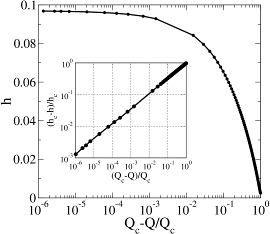
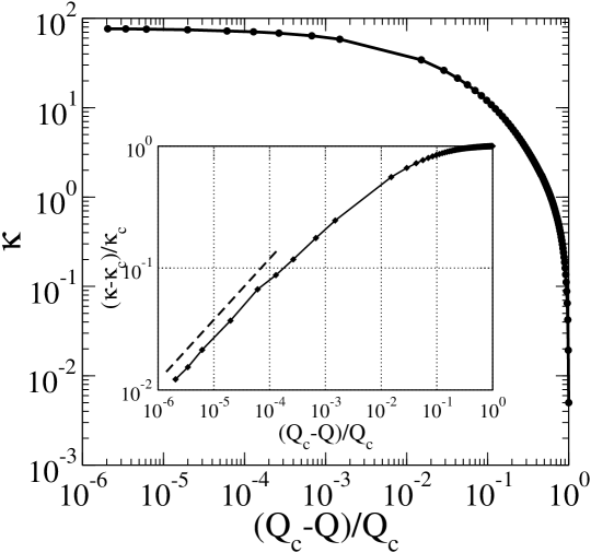
Figure 4: Evolution of the calculated steady-state hump shape with withdrawal flux $Q$. (a) Hump height $h$ vs. $Q_{c}-Q/Q_{c}$. The inset shows $(h_{c}-h)/h_{c}$ approaches saturation as $\sqrt{(Q_{c}-Q)/Q_{c}}$. (b) Mean curvature $\kappa$ at hump tip versus $Q$. The inset shows $(\kappa_{c}-\kappa)/\kappa_{c}$ approaches saturation as $\sqrt{(Q_{c}-Q)/Q_{c}}$. The dashed line depicts a square root powerlaw.

 

The observed square-root dependence of $h_{c}-h$ and $\kappa_{c}-\kappa$ suggests that the transition from selective withdrawal to viscous entrainment occurs via a collision at $Q_{c}$ of two steady-state hump solutions, one stable and one unstable. In other words, the transition from selective withdrawal to viscous withdrawal has the structure of a saddle-node bifurcation. Typically, saddle-node bifurcations are associated with solutions that remain smooth at the bifurcation point. Therefore the observed square-root scaling suggests that the final evolution of the interface as the transition is approached is not organized by an approach towards a singular steady-state shape.

The saddle-node structure of the transition can be rationalized by considering the flow in the upper layer converges along the centerline and therefore speeds up away from the tip of the hump. Since the hump solution is realized in a time-dependent simulation and also observed in the experiment, it is linearly stable. We therefore expect that small upwards perturbations of the hump tip simply decay downwards as the hump shape relaxes towards the steady-state solution over time. However, if the upwards perturbation is very large, so that the perturbed hump tip now lies very close to the sink, then surface tension effects will be too weak to pull the perturbed interface downwards. Instead, the hump tip will be drawn into the sink. This suggests there exists an intermediate critical shape perturbation that neither decays nor grows upwards but simply remains steady over time, as illustrated in figure 5a. This critical shape perturbation would correspond to an unstable hump solution.

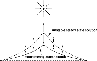
Figure 5: (a) Stable and unstable hump solutions in steady-state selective withdrawal. (b) Saddle-node bifurcation diagram illustrating the evolution of the hump curvature in the selective withdrawal regime.

 

Figure 5b illustrates the evolution of the hump curvature as a function of the flow rate for stable and unstable hump solutions. At low withdrawal flux values, only a very large shape perturbation can cause the interface to be drawn into the sink, we therefore expect the stable and the unstable hump shapes to be widely separated. This means the unstable hump must lie close to the sink and, as a result, has a very curved tip. At moderate withdrawal flux values, the perturbation size required to destabilize the hump solution becomes smaller, implying that the unstable and stable solutions now lie closer to each other. Concurrently, the curvature of the stable solution increases, and the curvature of the unstable solution decreases. Near transition, even a small perturbation causes the interface to become unstable and grow towards the sink. This suggests that the two solutions lie very close each other and are nearly identical. Therefore it is very reasonable to expect the two solutions to become identical, or coincide, at $Q_{c}$, thereby bringing about a saddle-node bifurcation of the hump solution. The square-root scaling corresponds to a smooth merging of the two solutions, so that the $\kappa(Q)$ curve at $Q_{c}$ has a shape of a parabolic lying on its side.

The scaling dynamics associated with how the hump solution saturates as $Q$ approaches $Q_{c}$ is consistent with a saddle-node bifurcation at $Q_{c}$. This is a generic mechanism for transition for one type of solution from another in a nonlinear problem. However, the quantitative analysis in figure 4 shows one surprising and atypical feature: the hump height and curvature saturate towards the final scaling behavior at very different $\delta q$ values. Specifically, the square-root scaling in $h_{c}-h$ is evident throughout its evolution, even at large $\delta q$. In contrast, the square-root scaling for $\kappa_{c}-\kappa$ becomes evident only when $\delta q$ has decreased below $10^{-3}$. This behavior suggests that the hump shape does not approach the transition uniformly. To test this idea we plot the hump radius at $z=h/2$ as a function of $Q$ in figure 6. We find that the radius at the half-height saturates to the final scaling behavior later than $h$, but earlier than $\kappa$ as $\delta q$ approaches $0$. This behavior indicates that, as $Q$ approaches $Q_{c}$, the overall shape of the hump, e.g. the hump height or its lateral extent, saturates first, followed by features on smaller lengthscales. The shape of the hump at its tip, which corresponds to a feature on the smallest lengthscale, saturates last. This cascade of events is more typical of an approach towards a singular shape, in which the evolution of features on different lengthscales are nearly decoupled, so that features on smaller lengthscales saturate later than features on large lengthscales.

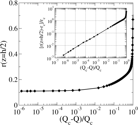
Figure 6: Evolution of the hump radius at $z=h/2$ as a function of the withdrawal flux $Q$. The inset shows how the radius at half height reaches its saturation value.

 

To get some insight into this unusal hybrid character of the interface evolution near transition, we plot $\kappa$ as a function of $h$ in figure 7. At $Q=0$, the interface shape is given by a balance of Laplace pressure and reservoir pressure $p_{0}$. For $p_{0}=0.01$, the shape is a nearly flat spherical cap. When the interface is only weakly perturbed from the $Q=0$ shape, both $\kappa$ and $h$ increase linearly with $Q$, and therefore $\kappa\propto h$. This linear regime persists until $h\approx 0.02$. Beyond this point, $\kappa$ increases much more rapidly than $h$. Remarkably, this large increase of $\kappa$ relative to the increase in $h$ is well-approximated by a simple mathematical expression, as evident from the inset for figure 7. In the nonlinear deflection regime,

$$\ln(\kappa)\propto h\ .$$ (20)

This logarithmic coupling indicates that in the nonlinear regime, the hump solution evolves so that small increases in hump height corresponds to large increases in the hump curvature. This does not correspond to a nearly continuous transition, as suggested by Cohen & Nagel (Cohen & Nagel (2002)), since the hump curvature $\kappa$ never decouples from the hump height. Instead, our results show that $\kappa$ remains weakly coupled to $h$ and does not diverge as the tranisiton is approached. To gain some insights into the origin of this unusual coupling, we next investigate how changes in the withdrawal conditions, in particular the sink height $S$ and the reservoir pressure $p_{0}$, affect this relation between the hump curvature and the hump height.

Figure 7: Mean curvature at the hump tip versus the hump height. Inset shows the same data on a semi-log plot. When the deflection is sufficently large, the hump height $h$ has a linear dependence on $\ln(\kappa)$.

 

4.2 Interface Evolution under Different Withdrawal Conditions

Naively one may expect that a logarithmic coupling between the hump height and the hump curvature would be easily perturbed by changes in the boundary conditions, since logarithmic coupling is often observed at the transition between different kinds of power-law scaling as some system parameter is varied. In addition the withdrawal process analyzed numerically is highly idealized and may therefore give results which are not generic. To address these concerns, we analyze numerical results for the steady-state interface shapes under a variety of withdrawal conditions. Surprisingly, we find the logarithmic coupling (20) to be a robust feature of equal-viscosity selective withdrawal in all the numerical solutions.

To determine the effect of the reservoir pressure $p_{0}$ on the transition structure we analyzed the numerical solutions for values of $p_{0}$ ranging from $-0.3$ to $0.3$. Larger $p_{0}$ values were not investigated because they result in static shapes whose height is greater than the sink height even at $Q=0$. In figure 8 we plot $\kappa_{c}$ and $h_{c}$, the hump curvature and hump height at transition versus $p_{0}$. We find that the precise value of $p_{0}$ makes little difference to the values of $\kappa_{c}$ and $h_{c}$. Also, all the runs show the same logarithmic dependence of $\kappa$ on $h$ near the transition.

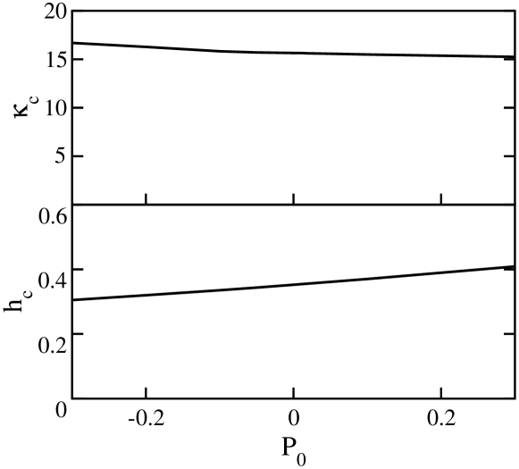
Figure 8: Calculated hump curvature $\kappa_{c}$ and hump height $h_{c}$ at transition as a function of the reservoir pressure $p_{0}$. The sink height $S=1$.

 

In contrast, figure 9 shows that varying the sink height $S$ strongly affects $\kappa_{c}$ and $h_{c}$. As the dimensionless sink height $S$ becomes much smaller than $1$, or $\tilde{S}\ll a$, the hump curvature at transition, $\kappa_{c}$, increases as $1/S$ while $h_{c}$ decreases as $S$. In the opposite limit, as $S$ becomes much larger than $1$, or $\tilde{S}\gg a$, both $\kappa_{c}$ and $h_{c}$ approach constant values. These trends can be understood by analyzing the limiting cases where the sink is either very far or very near to the interface. When the sink is placed very close to the interface, the effect of the pinning at $a$ becomes irrelevant since the interface is already flat at distances $O(S)$ where the flows become very weak. Consequently, $h_{c}$ and $\kappa$ only depend on $S$ when $S\ll 1$. In the opposite limit, where $\tilde{S}\gg a$, the flow at the interface becomes almost uniform because the lengthscale over which the imposed withdrawal flow varies is much larger than $a$. Under these conditions the interface shape is primarily determined by the pinning condition at $a$ and is insensitive to changes in the sink height.

Figure 9 also shows that the variation in $\kappa_{c}$ tracks the variation in $h_{c}$ almost perfectly as $S$ is varied. Consequently, even though driving the withdrawal with a sink closer to the interface produces a larger hump curvature at transition, it does not prduce a sharper hump tip. This is because the hump height, and similarly the overall deformation at transition, is proportionally smaller as well, so that the product $\kappa_{c}\cdot h_{c}$ characterizing the relative separation of lengthscale between the hump tip and the hump height remains roughly constant with $S$. Changing the sink height primarily changes the absolute lengthscale of the steady-state deformation at the onset of entrainment. It does not change the shape of the deformation significantly.

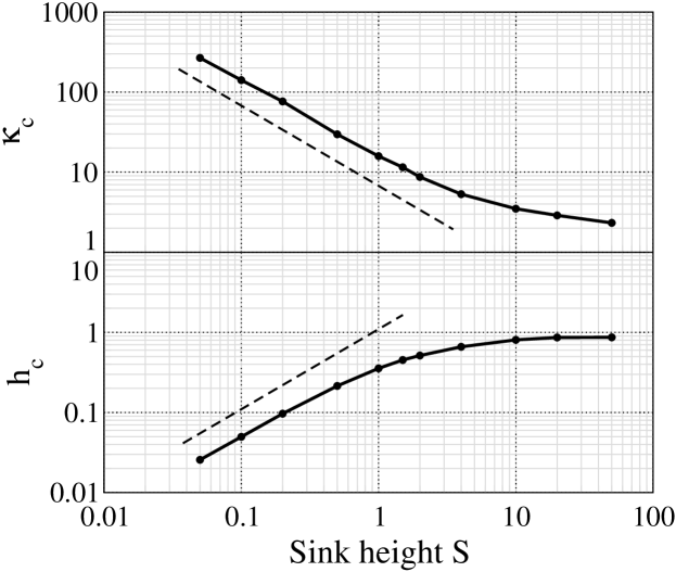
Figure 9: Calculated hump curvature $\kappa_{c}$ and hump height $h_{c}$ at transition different sink heights $S$. The reservoir pressure $p_{0}=0.01$. The dashed line in the $\kappa_{c}$ vs. $S$ plot shows a $1/S$ dependence. The dashed line in the $h_{c}$ vs. $S$ plot shows a $S$ dependence.

 

This observation suggests that dividing all lengths by $h_{c}$ should scale out most of the variation observed at different sink heights. In figure 10 we plot $h_{c}\cdot\kappa$ versus $h/h_{c}$ obtained from numerical solutions where $S=0.05$, $0.2$, $1$, $10$ and $50$ representing a $10^{3}$ variation in the sink height. We find that the curves are indeed brought close together by this rescaling. For example, while the actual value of $\kappa_{c}$ changes by a factor of $100$ between $S=0.05$ and $S=50$, the rescaled value $h_{c}\cdot\kappa_{c}$ changes by less than a factor of $4$. We do however, observe small changes in the slope and intercept of the logarithmic curves even when $\kappa$ and $h$ are rescaled. Nevertheless, from these results, we conclude that the logarithmic coupling is a robust feature of our idealized model of two-layer withdrawal. Changing either the boundary condition parameter $p_{0}$, or the forcing parameter $S$ within the simple model of withdrawl produces no qualitative change in the evolution of the steady-state hump shape as a function of the withdrawal flux.

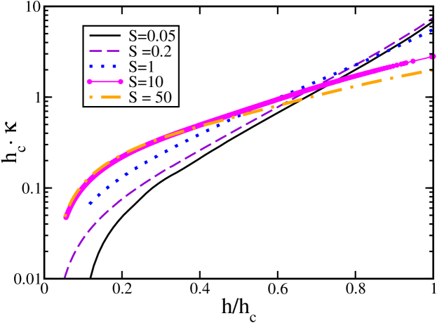
Figure 10: Calculated hump curvature $\kappa$ versus hump height $h$ at $S=0.05$, $0.2$, $1$, $10$ and $50$.

 

Given this robustness with respect to variation in system parameters in the simple model, we next analyze the steady-state interface obtained under different realizations of selective withdrawal. We find that even these different realizations, which correspond to different boundary conditions and/or imposed withdrawal flows, fail to produce a qualitative change in how the steady-state hump shape evolves. Figure 11 shows the interface shapes obtained in two different sets of calculations, each with a lower layer of finite depth, instead of the infinite depth assumed in the model calculation. In the first case, the lower layer is contained in a cylindrical cell of radius $a_{1}$ and depth $a_{1}$ (figure 11a). This corresponds to a situation where the lower-layer is confined equally in both the radial and vertical direction. The toroidal recirculation established in the lower-layer is therefore much smaller in extent, thereby resulting in an $O(1)$ change in the viscous stresses exerted on the interface by the flow in the lower layer.

Figure 11: (a) Steady-state interface shapes obtained in selective withdrawal from a lower layer of finite depth. The cell depth equals the cell radius $a_{1}$ and the sink height $\tilde{S}/a_{1}=0.5$. (b) Steady-state interface shapes obtained in selective withdrawal from a thin lower-layer overlying a solid plate of radius $a_{2}$. The sink height $\tilde{S}/a_{2}=0.2$.

 

For this realization, the boundary integral formulation uses a closed surface comprised of the liquid interface $S_{I}$, the side walls of the container $S_{\textrm{side}}$ and the bottom wall of the containter $S_{b}$. The disturbance velocity $\mathbf{u}$ on the interface is given by

$$\frac{1}{2}\mathbf{u}(\mathbf{x}) = \int_{S_{I}}\mbox{\boldmath$J$}\cdot\mathbf{n}\left[\gamma 2\tilde{\kappa}\right]\,\rm dS_{\mathbf{y}}+\int_{S_{\textrm{side}}}\mbox{\boldmath$J$}\cdot\mathbf{n}\ \mbox{\boldmath$\sigma$}_{\textrm{side}}\,\rm dS_{\mathbf{y}}$$

$$+ \int_{S_{\textrm{b}}}\mbox{\boldmath$J$}\cdot\mathbf{n}\ \mbox{\boldmath$\sigma$}_{\textrm{b}}\,\rm dS_{\mathbf{y}}\quad\textrm{ for }\mathbf{x}\in S_{I}$$

where $\mathbf{y}$ is the point on the surface that you are integrating over, $\mbox{\boldmath$\sigma$}_{\textrm{side}}$ and $\mbox{\boldmath$\sigma$}_{\textrm{b}}$ correspond to the normal stress exerted by the flow on the side wall and bottom wall of the container. The two stresses are found by solving the equation

$$\mathbf{0} = \int_{S_{I}}\mathbf{J}\cdot\mathbf{n}\left[\gamma 2\tilde{\kappa}\right]\,\rm dS_{\mathbf{y}}+\int_{S_{\textrm{side}}}\mathbf{J}\cdot\mathbf{n}\cdot\mbox{\boldmath$\sigma$}_{\textrm{side}}\,\rm dS_{\mathbf{y}}$$

$$+ \int_{S_{\textrm{b}}}\mbox{\boldmath$J$}\cdot\mathbf{n}\cdot\mbox{\boldmath$\sigma$}_{\textrm{b}}\,\rm dS_{\mathbf{y}}\quad\textrm{ for }\mathbf{x}\in S_{\textrm{side}}\textrm{ or }S_{\textrm{b}}.$$

This corresponds to enforcing no-slip boundary conditions on the side walls and the bottom walls of the container.

The interface shapes shown are the calculated results and the cell radius $a_{1}$ is used as a characteristic lengthscale in nondimensionalizing various quantities. As the withdrawal flux $Q$ increases and the hump height increases, liquid is drawn from the lower layer into the hump. Since volume in the lower layer is conserved, gathering extra liquid into the hump forces a shallow dip in the interface shape to develope some distance away from the centerline. Thus, the hump profile no longer flattens monotonically with $r$, in contrast to results obtained assuming an infinitely deep lower layer. However, these qualitative changes to the overall shape do not significantly change how the interface evolves with $Q$. The shape transition still corresponds to a saddle-node bifurcation (figure 12). A comparison of the rescaled $h_{c}\cdot\kappa$ versus $h/h_{c}$ curve obtained for a cell of finite depth and the analogous curve obtained assuming an infinitely deep layer in figure 13 show the same trend.

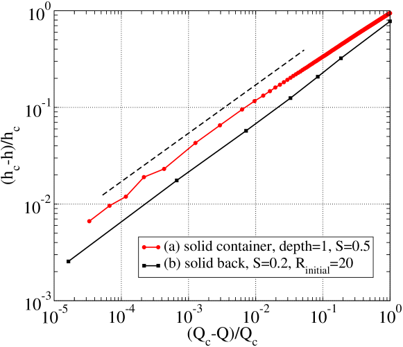
Figure 12: Scaling of the calculated hump height $h$ near the transition flow rate for two-layer withdrawal. Set (a) corresponds to withdrawal from a cylindrical container. Set (b) corresponds to withdrawal from a thin lower layer which is resting on a solid plate.

 

Figure 11b shows what happens when we change the condition in the lower layer more drastically. In this set of calculation, a thin layer of the lower layer liquid overlies a solid plate. The plate radius $a_{2}$ is used as a characteristic lengthscale in the nondimensionalization. The liquid is assumed to wet the solid substrate so that the plate is covered by liquid from the lower-layer at all $Q$. The formation of a hump causes most of the liquid in the layer to drain into the hump, leaving only a very thin layer covering the rest of the solid plate. In the selective withdrawal regime, the withdrawal flow requires liquid in the lower layer to recirculate, moving along the interface towards the hump and then along the lower solid surface away from the hump. When the lower layer is thin, the viscous resistance associated with the steady-state recirculation is amplified dramatically. In this realization, therefore, the stress-balance on the steady-state interface is strongly perturbed from that obtained for withdrawal with an infinitely deep lower layer.

For two-layer withdrawal with a thin layer of the lower liquid, the closed surface used in the boundary integral formulation consists of the liquid interface $S_{I}$ and the bottom wall of the containter $S_{b}$. The equation for the velocity on the interface has the same form as (4.2) except that the terms associated with the side wall surface $S_{\textrm{side}}$ are absent. The normal stress on the solid surface $\sigma_{\textrm{b}}$ satisfies equation (4.2), without the sidewall contribution.

Comparing against results from the simple model and results for withdrawal from a finite container, we can see that reducing the thickness of the lower layer has an effect on the steady-state shape of the interface obtained. The hump shape is significantly more conical, and the flattening of the interface at large $r$ results primarily from volume conservation, rather than pinning at $a_{2}$ or the decay of the imposed withdrawal flow away from the sink. However, as evident from figure 12 and figure 13, the qualitative features are unchanged. The transition still corresponds to a saddle-node bifurcation. The evolution of the hump height $h$ retains a logarithmic coupling to the hump curvature $\kappa$. The main difference between withdrawal from an infinitely deep layer and withdrawal from a very thin layer overlying a solid plate is a shift in the slope of the rescaled $\kappa$ versus $h$ curve.

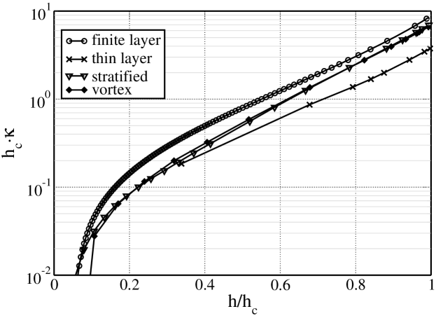
Figure 13: Curvature versus hump height under different withdrawal conditions. Open circles correspond to withdrawal with a lower layer of finite depth contained in a cylindrical cell. The cell depth equals the cell radius $a_{1}$ and the sink height $\tilde{S}/a_{1}=0.5$. The crosses correspond to withdrawal of a thin layer of liquid overlying a solid plate of radius $a_{2}$ and sink height $\tilde{S}/a_{2}=0.2$. The open triangles correspond to withdrawal from a stratified layer. The capillary lengthscale $\ell_{\gamma}/a=0.1$ and the rescaled sink height is $0.2$. The solid diamonds correspond to withdrawal driven by a vortex ring of radius $a_{\omega}=a$, dimensionless strength $\omega$ and height $\tilde{S}/a=0.2$. The $\kappa$-$h$ curve obtained for $S=0.2$ and $p_{0}=0.01$ (solid line) is also shown for comparison.

 

We have also conducted a series of calculations which include the effect of hydrostatic pressure explicitly. This requires that we change the form of the normal stress jump $[\mathbf{n}\cdot\mbox{\boldmath$\sigma$}]_{-}^{+}$ across the liquid interface $S_{I}$ in the J-integral of equations (3.1) and (3.1) to

$$[\gamma 2\tilde{\kappa}-\Delta\rho\mathbf{g}\cdot\mathbf{y}]\mathbf{n}$$ (23)

where $\Delta\rho$ is the density difference between the two layers, $\mathbf{g}$ the gravitational acceleration and $\mathbf{y}$ the location of a point on the liquid interface. Choosing the capillary lengthscale $\ell_{\gamma}$ to be less than the pinning radius $a$ allows the interface to flatten out at large radial distances due to stratification, as occurs in the experiment, instead of due to the decay of the withdrawal flow or due to surface tenson effect. Results for $\ell_{\gamma}/a=0.1$ and $0.2$ show that introducing stratification explicitly results in slight qualitative changes in the hump shape but the same trend in the rescaled $\kappa$ versus $h$ curve (figure 13). Finally, to assess the influence of details of the geometry of the withdrawal flow on the logarithmic coupling (20), we changed the imposed withdrawal flow from a sink flow (2), to that associated with a vortex ring of size $a_{\omega}=a$ and strength $\omega_{0}$. The axisymmetric velocity field is given in terms of a stream function $\phi$

$$u_{r}=\frac{1}{r}\frac{\partial\phi}{\partial r}\qquad u_{z}=-\frac{1}{r}\frac{\partial\phi}{\partial z}$$ (24)

and the stream function has the form

$$\phi(r,z)=\frac{1}{4\pi}\int\int rr^{\prime}\omega(r^{\prime},z^{\prime})\rm dz^{\prime}\rm dr^{\prime}\int^{2\pi}_{0}\frac{\cos\theta\ \rm d\theta}{\sqrt{(z-z^{\prime})^{2}+r^{2}+r^{\prime 2}-2rr^{\prime}\cos\theta}}$$ (25)

where the vorticity distribution $\omega(r^{\prime},z^{\prime})$ has the form $\omega_{0}\delta(a_{\omega}-r)\delta(S-z^{\prime})$ for a vortex ring. This is a better approximation of the withdrawal flow imposed in the experiment, both because there is no net volume withdrawn and because the finite size of the vortex ring mimics the finite diameter of the tube. The rescaled $\kappa$ versus $h$ curve obtained from numerical solutions for withdrawal driven by a vortex ring again has the same logarithmic coupling between the hump height and the hump curvature near the transition.

In all the different realizations of selective withdrawal, the evolution of the steady-state interface approaches the form (20) for large deformations. As a result, $h_{c}\cdot\kappa_{c}$, the relative separation of lengthscales characterizing the hump shape at transition, changes little even when the forcing and/or the boundary conditions are changed drastically. In other words, regardless of what type of flow we use to drive the transition, the degree of viscous resistance from flow within the lower layer, or whether the interface flattens out on large lengthscale due to stratification or surface tension effects, the hump shape at transition never becomes significantly sharper than that first calculated in the simple model. We conclude from this that the interface shape at $Q_{c}$ produced in viscous withdrawal with two liquid layers of equal viscosity cannot be brought closer to a singular shape via changes in the boundary conditions. This contrasts sharply with theoretical results on viscous entrainment when the entrained liquid is far less viscous than the exterior, which show that interface shape at $Q_{c}$ can be made singular via changes in the boundary conditions (Zhang (2004)).

Finally, the robustness of the logarithmic coupling even under drastic changes in the withdrawal conditions suggests that (20) in fact corresponds to a generic feature of selective withdrawal from two layers of equal viscosity. This leads us to re-examine experimental measurements of $\kappa$ and $h$, previously interpretted in terms of a continous evolution towards a change in interface topology. In the next subsection we compare experimental results against numerical results obtained using the simplest model of withdrawal and show that the logarithmic coupling (20) is also a good description of the steady-state interface evolution in the experiments.

4.3 Comparison with Experiment

Here we compare three key results from the numerics against the measurement previously obtained by Cohen & Nagel (Cohen & Nagel (2002)). First, we analyze the $\tilde{h}(\tilde{Q})$ obtained in the experiment and show that the measurements are consistent with the interpretation that $h_{c}-h$ scales with $\sqrt{Q_{c}-Q}$ near the transition. Measurements of the hump curvature also agree well with the calculated values and begin to saturate as $Q_{c}$ is approached. Finally we compare the measured $\kappa$ versus $h$ curves against the calculation and show they also agree.

To make the comparison, we chose measurements from five different experiments, spanning the full range of tube heights used. Figure 14 shows how the measured hump height saturates as $Q$ approaches $Q_{c}$. As was done with the numerical results, in generating figure 14 we allowed ourselves to vary $h_{c}$ and $Q_{c}$ values within the experimental error bars, which are about $5\%$, in order to generate the best power-law fits for the measurements. For four sets of the data, the saturation behavior is completely consistent with a square-root scaling with $\delta q$. The set with the largest tube height ($S_{p}=0.830$ cm) shows a slight difference in the scaling behavior. We do not fully understand the origin of this discrepancy. We speculate that withdrawal experiments at larger tube heights require running the pump at higher flow rates. This may create more noise and/or signficant inertial effects, hence resulting in a discrepancy with experiments performed at lower tube heights. Overall the agreement shows that the hump height in the experiment experiences a saddle-node bifurcation at $Q_{c}$.

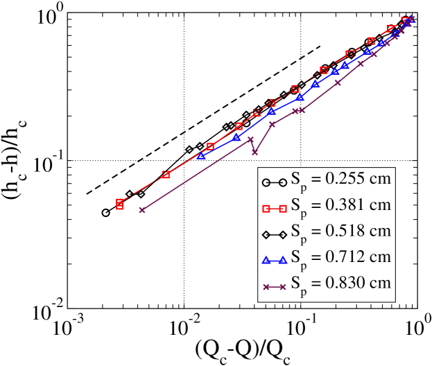
Figure 14: Rescaled hump heights $(h_{c}-h)/h_{c}$ versus rescaled withdrawal flux $(Q_{c}-Q)/Q_{c}$ for measurements obtained with $5$ different tube heights. The tube heights are $\tilde{S}_{p}=0.260$ cm, $0.381$ cm, $0.518$ cm, $0.712$ cm and $0.830$ cm. The capillary lengthscale in the experiment is $0.3$ cm and the layer viscosity ratio (lower/upper) is $0.86$. The calculation results are for $\tilde{S}/a=0.2$ and reservoir pressure $p=0.01$.

 

Next we compare measurements of the hump curvature against calculated values. Since the hump curvature satures at a much smaller value of $\delta q$, below the dynamic range of the experiment, we cannot compare the saturation dynamics, which is independent of the details of the numerical model, directly. Instead we compare the $\tilde{\kappa}(\delta q)$ curves obtained experimentally against the results obtained using our minimal numerical model, described in section 3.1, with $S\equiv\tilde{S}/a=0.2$. This is done in figure 15. The $Q_{c}$ values which produced the best power-law fit for the experimental data in figure 14 are used in figure 15. (More information on the difference between our analyses and those performed in the original papers (Cohen & Nagel (2002)) can be found in the appendix) As was done for numerical results obtained with different sink heights, we account for the change in the absolute size of the hump at different tube heights by rescaling $\tilde{\kappa}$ by $h_{c}$, the hump height at transition. This causes the different curves associated with different tube heights to collapse onto roughly a single curve. Significantly the collapsed curve shows some evidence of saturation as $\delta q$ approaches $0$. In order to display the comparison clearly, the range of value for both $\kappa\cdot h_{c}$ and $(Q_{c}-Q)/Q_{c}$ have been truncated. The calculated curve goes through the experimental values and shows exactly the same trend. Note that our choice of $S=0.2$ for the numerical results is primarily a matter of simplicity, since that is the set of results discussed in section 4.1. From section 4.2 we have seen that $\kappa_{c}\cdot h_{c}$ varies only weakly with $S$, so we could have used any $O(1)$ value for the dimensionaless sink height $S$ and gotten good agreement in this rescaled curvature plot. We conclude from the good agreement that the hump curvature also saturates in the experiment.

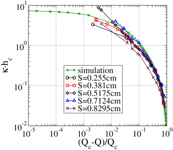
Figure 15: Tip curvature versus rescaled flow rate $\left(Q_{c}-Q\right)/Q_{c}$ for the numerical model and experimental data. The tip curvature has been non-dimensionalized by $h_{c}$. Range of the numerical results have been truncated to display the comparison clearly.

 

Finally we plot the rescaled measured hump curvature as a function of the rescaled hump height $h/h_{c}$ (Figure 16). The measurements at the largest tube height ($S_{p}=0.830$ cm) are displaced from the four other sets. Also, the measured curves for the three, larger tube heights show a slight but systematic upturn at large $h/h_{c}$, when compared against the calculated results. The two data sets for the lower tube heights appear to follow a logarithmic relation. While it is unclear what causes these discrepancies, overall there is good agreement between the calculated curve and the measured curves. The agreement shows that the simple model used here captures the main features in the evolution of the steady-state interface shape.

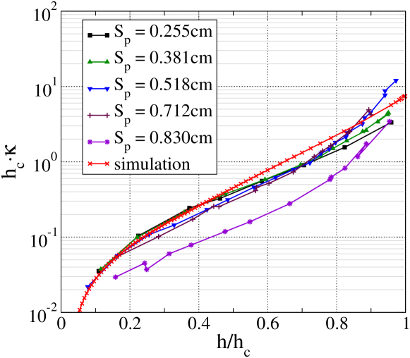
Figure 16: Comparison between measurements at five different pipette heights and calculation. Note the range of $\kappa\cdot h_{c}$ has again been truncated to display the overlap with measurements more clearly.

 

Previously, the large increase in the hump curvature near transition was interpretted in terms of the steady-state interface approaching a steady-state singularity as the withdrawal flux is increased (Cohen & Nagel (2002); Cohen (2004)). The good agreement between the numerical solutions and the experimental measurements show that this large increase in hump curvature can also be understood to result from a weak coupling between the overall hump shape, characterized by the hump height, and the shape of the hump tip, characterized by the hump curvature. The simplest way to account for all the results, numerical and experimental, obtained for equal-viscosity withdrawal is to assume that no singular hump solution exists for equal-viscosity withdrawal and that the logarithmic coupling (20) is a generic feature of selective withdrawal. The absence of a singular solution for equal-viscosity withdrawal would explain why even drastic changes in the withdrawal conditions failed to introduce qualitative changes in the $\kappa$ versus $h$ curves calculated, and why the product $\kappa_{c}\cdot h_{c}$ characterizing the sharpness of the hump profile always remains below $20$. The saddle node structure of the transition and the logarithmic coupling between $h$ and $\kappa$ also account in a natural way for the two features which appear puzzling in the context of a nearly continuous shape transition: the apparent transition cut-off in the hump evolution and the large changes in the hump curvature relative to changes in hump height.

While our results simplify the view of the steady-state interface evolution significantly, they do not offer a full explanation. We do not know why the logarithmic coupling should arise in selective withdrawal in the first place. Section 5 offers a brief, and speculative, discussion of its possible origin, focusing in particular on a comparison between previously proposed singular solutions and the logarithmic relation found in our numerical solution.

5 Discussion

A natural way to reconcile the logarithmic evolution of the hump height relative to hump curvature (20) obtained here with the previously proposed idea that the sharpening of the steady-state hump tip is associated with an approach towards a steady-state singularity is to suppose that the interface evolution is indeed organized by the existence of a steady-state singularity, as suggested by previous studies. However, the singular shape is not nearby in the sense that it is attained at $Q$ just above $Q_{c}$, where a transition from selective withdrawal to viscous entrainment takes place. Instead, the singular solution corresponds to an isolated singularity, existing at a value $Q_{*}$ much larger than $Q_{c}$. Correspondingly, the height of the singular hump $h_{*}$, is much larger than $h_{c}$, the hump height at transition. In other words, the steady-state interface evolves towards a singular shape at $Q_{*}$ as the withdrawal flux is increased. However, this evolution is cut-off at a withdrawal flux $Q_{c}$ far below $Q_{*}$ by a saddle-node bifurcation. While unusual, a steady-state cusp solution corresponding to an isolated singularity has been found for 2D selective withdrawal of inviscid fluid (Tuck & Vanden-Broeck (1984)) so this is a possible scenario for the steady-state evolution.

Under these assumptions, the power-law scaling

$$\frac{\kappa}{C}=\left(\frac{h_{*}}{h_{*}-h}\right)^{\beta}$$ (26)

where $C$ is a characteristic curvature scale, indeed assumes an approximate logarithmic form. Since $h_{c}\ll h_{*}$, the ratio $h/h_{*}$ is small over the entire range. Taylor series expansion of the natural log of (26) yields

$$\ln\left(\frac{\kappa}{C}\right)=-\beta\ln\left(1-\frac{h}{h_{*}}\right)=\beta\left(\frac{h}{h_{*}}+\frac{1}{2}\left(\frac{h}{h_{*}}\right)^{2}+\cdot\cdot\cdot\right)\ .$$ (27)

When $h_{c}/h_{*}$ is sufficiently small, the higher order terms are negligible, and we obtain a logarithmic relation between $\kappa$ and $h$

$$\ln\left(\frac{\kappa}{C}\right)=\left(\frac{\beta h_{c}}{h_{*}}\right)\frac{h}{h_{c}}\ .$$ (28)

According to Cohen & Nagel, the singular shape is characterized by a scaling exponent $\beta$ between $0.75$ and $0.82$ (Cohen & Nagel (2002)). In the long-wavelength analysis of spout formation (Zhang (2004)), Zhang found that the steady-state spout shape approaches a singular, conical shape. This would correspond to $\beta=1$. More recently, experimental and scaling analysis by Courrech du Pont and Eggers show that the cusp observed in a viscous drainage experiment approaches a conical shape (Courrech du Pont & Eggers (2006)), with $\beta=1$. Given these values, consistency requires that the coefficient $\beta h_{c}/h_{*}$ must be much smaller than $1$, since (28) is derived under the assumption that $h_{c}/h_{*}\ll 1$. We can check this against the numerical results by fitting the calculated $\kappa$ versus $h$ curves with the form

$$\ln\left(\frac{\kappa}{\kappa_{0}}\right)=b\left(\frac{h}{h_{c}}\right)$$ (29)

where $\kappa_{0}$ is the extrapolated intercept at $h=0$ and the slope $b=\beta h_{c}/h_{*}$ in (28). Fits to the calculated curves for $S=0.05$, $0.2$ and $50$ yield, respectively, $b$ values $5.5$, $5.9$, and $1.9$, all above $1$. Consequently, $h_{c}/h_{*}$ is $O(1)$ which invalidates the Taylor expansion in equation (27). This clearly rules out the possibility that the logarithmic relation reflects the existence of an isolated singular hump solution for equal-viscosity withdrawal.

A number of future studies would complement this one. It would be useful to explicitly calculate the unstable hump solution, given its relation with the stability of the hump solutions. In light of recent works (Chaieb (2004); Zhang (2004); Courrech du Pont & Eggers (2006)) suggesting that the steady-state interface indeed evolves towards a singular shape when the lower layer is much less viscous than the upper layer, it would also be worthwhile to analyze the selective withdrawal regime when the two liquid layers have unqual viscosities. We expect that the final transition from selective withdrawal to viscous entrainment occurs via a saddle-node bifurcation even when the liquid layers have unequal viscosities. However, the limiting situation where the lower layer has a vanishingly small viscosity relative to the upper layer corresponds to a qualitative change in the entrainment dynamics since only the flow in the upper layer is significant. This then suggests a qualitative change in the steady-state shape evolution as well.

6 Conclusion

In conclusion, this paper presents a numerical study of a simple example of flow-driven topological transition: the transition from selective withdrawal to viscous entrainment. To uncover the fundamental nature of the topology change, we focus on the selective withdrawal regime, and analyze how the steady-state shape of an interface between two immiscible and viscous liquid layers changes as the imposed flow strength increases. We analyze a model problem in which the interface deformation is solely controlled by viscous stresses and surface tension. Its results show that the hump solution corresponding to the selective withdrawal regime experiences a saddle-node bifurcation at a threshold flow rate. Above the threshold, no hump solution exists. As observed in the experiments, the hump curvature increases dramatically near transition while the hump height increases only weakly, but the increase corresponds to a logarithmic coupling between the hump height and the hump curvature. This suggests that the evolution of the hump tip remains weakly coupled with the evolution of the overall hump shape as the transition is approached. Moreover, we find that this logarithmic coupling is robust. Numerical solutions for different realizations of viscous withdrawal, as well as measurements, all show a logarithmic coupling between hump height and hump curvature.

Appendix A

As was seen in previous sections, compared to the hump height, the tip curvature shows evidence of saturation towards a final value only when $Q$ is very close to $Q_{c}$. As a consequence, when the entrainment threshold is approached, the tip curvature can appear to diverge while the hump height reaches a saturation value. In particular, when $\kappa$ is plotted against $(Q_{c}-Q)/Q$ instead of $(Q_{c}-Q)/Q_{c}$, it is very difficult to distinguish between a continued power law and a turn over into saturation with the available range of experimental data. This is because even a slight shift in the value of $Q_{c}$ can straighten out the curves. The apparent power law in the $(Q_{c}-Q)/Q$ range between $1$ and $10^{-2}$ seems to be an artifact of the fact that, when $Q$ is small, the denominator of $\left(Q_{c}-Q\right)/Q$ is close to $Q_{c}$ and almost constant, thus the entire expression scales roughly like $1/Q$. Furthermore, for small flow rates $Q$ the system response to the outside flow can be assumed to be almost linear, with a linear dependence of $\kappa$ on $Q$. This would then asymptotically give rise to a powerlaw with an exponent of $-1$.

Figure 17: Tip curvature versus rescaled flow rate $\left(Q_{c}-Q\right)/Q$ for the numerical model and experimental data. The tip curvature has been non-dimensionalized using the threshold hump height $h_{c}$. Errors in the experimental tip curvature were estimated to be approximately 10%. The model system parameters are $S=0.2$, $p_{0}=0.01$.

References

- Acrivos & Lo (1978) Acrivos, A. & Lo, T. S. 1978 Deformation and breakup of a single slender drop in an extensional flow. J. Fluid Mech. 86 (4), 641–672.
- Anna et al. (2003) Anna, S. L., Bontourx, N. & Stone, H. A. 2003 Formation of dispersions using flow focusing in microchannels. Appl. Phys. Lett. 82, 364–366.
- Blawzdziewicz et al. (2002) Blawzdziewicz, J., Cristini, V. & Loewenberg, M. 2002 Critical behavior of drops in linear flows. i. phenomenological theory for drop dynamics near critical stationary states. Physics of Fluids 14 (8), 2709–2718.
- Buckmaster (1973) Buckmaster, J. D. 1973 The bursting of pointed drops in slow viscous flow. J. Appl. Mech. E 40, 18–24.
- Case & Nagel (2006) Case, S. C. & Nagel, S. R. 2006 Spout states in the selective withdrawal system. ArXiv:cond-mat/0608140.
- Chaieb (2004) Chaieb, S. 2004 Free surface deformation and cusp formation during the drainage of a very viscous fluid. ArXiv:physics/0404088.
- Cohen (2004) Cohen, I. 2004 Scaling and transition structure dependence on the fluid viscosity ratio in the selective withdrawal transition. Phys. Rev. E 70, 026302.
- Cohen et al. (1999) Cohen, I., Brenner, M. P., Eggers, J. & Nagel, S. R. 1999 Two fluid snap-off problem: experiments and theory. Phys. Rev. Lett. 83 (6), 1147–1150.
- Cohen et al. (2001) Cohen, I., Li, H., Hougland, J. L., Mrksich, M. & Nagel, S. R. 2001 Using selective withdrawal to coat microparticles. Science 292, 265–267.
- Cohen & Nagel (2002) Cohen, I. & Nagel, S. 2002 Scaling at the selective withdrawal transition through a tube suspended above the fluid surface. Phys. Rev. Lett. 88 (7), 074501.
- Doshi et al. (2003) Doshi, P., Cohen, I., Zhang, W. W., Siegel, M., Howell, P., Basaran, O. A. & Nagel, S. R. 2003 Persistence of memory in drop breakup: The breakdown of universality. Science 302, 1185–1188.
- Eggers (1997) Eggers, J. 1997 Nonlinear dynamics and breakup of free-surface flows. Rev. Mod. Phys. 69 (3), 865–929.
- Eggers (2001) Eggers, J. 2001 Air entrainment through free-surface cusps. Phys. Rev. Lett 86 (19), 4290–4293.
- Eggers et al. (1999) Eggers, J., Lister, J. R. & Stone, H. A. 1999 Coalescence of liquid drops. J. Fluid Mech. 401, 293–310.
- Forbes et al. (2004) Forbes, L. K., Hocking, G. C. & Wotherspoon, S. 2004 Salt-water up-coning during extraction of fresh water from a tropical island. J. Eng. Math. 48, 69–91.
- Grace (1982) Grace, P. 1982 Dispersion phenomena in high viscosity immiscible fluid systems and application of static mixers as dispersion devices in such systems. Chem. Eng. Commun. 14, 225–239.
- Hocking & Forbes (2001) Hocking, G. C. & Forbes, L. K. 2001 Super-critical withdrawal from a two-layer fluid through a line sink if the lower layer is of finite depth. J. Fluid Mech. 428, 333–348.
- Imberger & Hamblin (1982) Imberger, J. & Hamblin, P. F. 1982 Dynamics of lakes, reservoirs and cooling ponds. Ann. Rev. Fluid Mech. 14, 153–187.
- Ivey & Blake (1985) Ivey, G. N. & Blake, S. 1985 Axisymmetrical withdrawal and inflow in a density-stratified container. J. Fluid Mech. 161, 115–137.
- Jellinek & Manga (2002) Jellinek, A. M. & Manga, M. 2002 The influence of a chemical boundary layer on the fixity, spacing and lifetime of mantle plumes. Nature 418, 760–763.
- Jeong & Moffatt (1992) Jeong, J.-T. & Moffatt, H. K. 1992 Free-surface cusps associated with flow at low reynolds number. J. Fluid Mech. 241, 1–22.
- Joseph et al. (1991) Joseph, D. D., Nelson, J., Renardy, M. & Renardy, Y. 1991 Two-dimensional cusped interfaces. J. Fluid. Mech. 223, 383–409.
- Ladyzhenskaya (1963) Ladyzhenskaya, O. A. 1963 The Mathematical Theory of Viscous Incompressible Flow. New York: Gordon and Breach Science Publishers.
- Lee & Leal (1982) Lee, S. H. & Leal, L. G. 1982 The motion of a sphere in the presence of a deformable interface. ii. a numerical study of the translation of a sphere normal to an interface. J. Colloid. Interface Science 87, 81–106.
- Limat & Stone (2004) Limat, L. & Stone, H. 2004 Three-dimensional lubrication model of a contact line corner singularity. Europhys. Lett. 65, 365–371.
- Link et al. (2004) Link, D. R., Anna, S. L., Weitz, D. A. & Stone, H. A. 2004 Geometrically mediated breakup of drops in microfluidic devices. Phys. Rev. Lett. 92, 054503.
- Lister (1989) Lister, J. R. 1989 Selective withdrawal from a viscous two-layer system. J. Fluid Mech. 198, 231–254.
- Lorenceau et al. (2004) Lorenceau, E., Quere, D. & Eggers, J. 2004 Air entrainment by a viscous jet plunging into a bath. Phys. Rev. Lett. 93, 254501.
- Lorenceau et al. (2003) Lorenceau, E., Restagno, F. & Quere, D. 2003 Fracture of a viscous liquid. Phys. Rev. Lett. 90 (184501).
- Lorenceau et al. (2005) Lorenceau, E., Utada, A. S., Link, D. R., Cristobal, G., Joanicot, M. & Weitz, D. A. 2005 Generation of polymerosomes from double-emulsions. Langmuir 21, 9183–9186.
- Lorentz (1907) Lorentz, H. A. 1907 Ein allgemeiner satz, die bewegung einer reibenden flüssigkeit betreffend, nebst einigen anwendungen. Abhandl. üb. theor. Physik 1, 23.
- Lubin & Springer (1967) Lubin, B. T. & Springer, G. S. 1967 Formation of a dip on surface of a liquid draining from a tank. J. Fluid Mech. 29, 385–389.
- Miloh & Tyvand (1993) Miloh, T. & Tyvand, P. A. 1993 Nonlinear transient free-surface flow and dip formation due to a point sink. Phys. Fluids A 5, 1368–1375.
- Navot (1999) Navot, Y. 1999 Critical behavior of drop breakup in axisymmetric viscous flow. Phys. Fluids 11, 990–996.
- Oddershede & Nagel (2000) Oddershede, L. & Nagel, S. R. 2000 Singularity during the onset of an electrohydrodynamic spout. Phys. Rev. Lett. 85.
- Oguz & Prosperetti (1990) Oguz, H. N. & Prosperetti, A. 1990 Bubble entrainment by the impact of drops on liquid surfaces. J. Fluid Mech. 219, 143–179.
- Courrech du Pont & Eggers (2006) Courrech du Pont, S. & Eggers, J. 2006 Tip singularity on a liquid-gas interface. Phys. Rev. Lett. 96, 034501.
- Pozrikidis (1992) Pozrikidis, C. 1992 Boundary integral and singularity methods for linearized viscous flow. Cambridge University Press.
- Rallison & Acrivos (1978) Rallison, J. M. & Acrivos, A. 1978 A numerical study of the deformation and burst of a viscous drop in an extensional flow. J. Fluid Mech. 89 (1), 191–200.
- Renardy & Renardy (1985) Renardy, M. & Renardy, Y. 1985 Perturbation analysis of steady and oscillatory onset in a bénard problem with two similar liquids. Phys. Fluids 28, 2699–2708.
- Renardy & Joseph (1985) Renardy, Y. & Joseph, D. D. 1985 Oscillatory instability in a bénard problem of two fluids. Phys. Fluids 28, 788–793.
- Sautreaux (1901) Sautreaux, C. 1901 Mouvement d’un liquide parfait soumis à lapesaneur. détermination des lignes de courant. J. Math. Pures Appl. 7, 125–159.
- Simpkins & Kuck (2000) Simpkins, P. & Kuck, V. J. 2000 Air entrapment in coatings by way of a tip-streaming meniscus. Nature 403, 641–643.
- Stokes et al. (2005) Stokes, T. E., Hocking, G. C. & Forbes, L. K. 2005 Unsteady flow induced by a withdrawal point beneath a free surface. Anziam J. 47, 185–202.
- Stone (1994) Stone, H. A. 1994 Dynamics of drop deformation and breakup in viscous fluids. Ann. Rev. Fluid Mech. 65, 65–102.
- Taylor (1934) Taylor, G. I. 1934 The formation of emulsions in definable fields of flow. Proc. Roy. Soc. A CXLVI, 501–523.
- Taylor (1964) Taylor, G. I. 1964 Conical free surfaces and fluid interfaces. Proc. 11th Int. Cong. Appl. Mech. pp. 790–796.
- Thoroddsen et al. (2005) Thoroddsen, S. T., Takehara, K. & Etoh, T. G. 2005 The coalescence speed of a pendant and a sessile drop. J. Fluid Mech. 527, 85–114.
- Tuck & Vanden-Broeck (1984) Tuck, E. O. & Vanden-Broeck, J. M. 1984 A cusp-like free-surface flow due to a submerged source or sink. J. Aust. Math. Soc. Ser. B 25, 443–450.
- Utada et al. (2005) Utada, A. S., Lorenceau, E., Link, D. R., Kaplan, P. D., A., S. H. & A., W. D. 2005 Monodisperse double emulsions generated from a microcapillary device. Science 308, 537–541.
- Vanden-Broeck & Keller (1987) Vanden-Broeck, J. M. & Keller, J. B. 1987 Free surface flow due to a sink. J. Fluid Mech. 175, 109–117.
- Wyman et al. (2004) Wyman, J., Dillmore, S., W., M., M., G., Mrksich, M. & R., N. S. 2004 Microencapsulation of islets of langerhans via selective withdrawal to achieve immunoisolation. APS March Meeting, W9.008.
- Zhang (2004) Zhang, W. W. 2004 Viscous entrainment from a nozzle: Singular liquid spouts. Phys. Rev. Lett. p. 184502.
- Zhang & Lister (1999) Zhang, W. W. & Lister, J. R. 1999 Similarity solutions for capillary pinch-off in fluids of differing viscosity. Phys. Rev. Lett. 83, 1151–1154.